\(\newcommand{\pder}[2]{\frac{\partial #1}{\partial #2}}\) \(\newcommand{\hpder}[2]{\dfrac{\partial #1}{\partial #2}}\) \(\newcommand{\eps}{\varepsilon}\) \(\newcommand{\beps}{\boldsymbol\varepsilon}\) \(\newcommand{\bsig}{\boldsymbol\sigma}\) \(\newcommand{\GAs}{GA_s}\) \(\newcommand{\ba}{\mathbf{a}}\) \(\newcommand{\bff}{\mathbf{f}}\) \(\newcommand{\bB}{\mathbf{B}}\) \(\newcommand{\bD}{\mathbf{D}}\) \(\newcommand{\bK}{\mathbf{K}}\) \(\newcommand{\xloc}{{\bar{x}}}\) \(\newcommand{\yloc}{{\bar{y}}}\)

4.3. 2D frame analysis

Frame structures are structures made of one-dimensional structural elements that are loaded axially as well as in bending. These structural elements can be considered a combination of the rod and the beam. One more conceptual ingredient needs to be added and that is that the structure is defined in two-dimensional space (or three-dimensional, but we limit the discussion to 2D here). This is different from rods and beams, which are 1D objects in 1D space. In a frame, different members are present that have different orientations, therefore a global coordinate frame is needed (see Fig. 4.2). In this chapter, we start with the formulation of an extensible beam element that is aligned with global coordinates. After that, we define the element for arbitrary orientation.

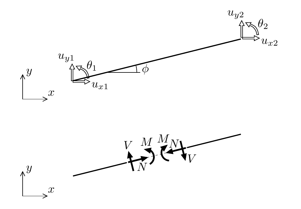
Fig. 4.2 The building block for 2D frame analysis: extensible beam element with three degrees of freedom per node and arbitrary orientation with respect to global coordinate frame

Extensible beam element

Governing equations

The extensible beam element is a combination of the rod element with a beam element. Here, we use a Timoshenko beam element. We take a linear 2-node element, initially one that is aligned with the global \(x\)-axis (\(\phi=0\) in Fig. 4.2). Notably, the same linear hat functions can be used as shape functions for rod elements as well as for Timoshenko beam elements, so in terms of shape functions, we need only one set. The same shape functions are used to interpolate three different fields (displacement-like quantities):

• the displacement in \(x\)-direction, \(u_x\), this is the \(u\) from rod analysis

• the displacement in \(y\)-direction, \(u_y\), this is the \(v\) from beam analysis

• and the rotation \(\theta\), also known from beam analysis

There are three deformations (strain-like quantities) that are related to these displacements with kinematic relations:

• axial strain \(\eps = \pder{u_x}{x}\)

• shear strain \(\gamma = \pder{u_y}{x}-\theta\)

• curvature \(\kappa = \pder{\theta}{x}\)

Then there are three section forces (stress-like quantities) that are related to the strains through constitutive relations:

• axial force \(N = EA\eps\)

• shear force \(V = \GAs\gamma\)

• moment \(M = EI\kappa\)

Where \(E\) is the Young’s modulus, \(A\) the cross-sectional area, \(I\) the second moment of inertia and \(\GAs\) the shear stifness (shear modulus times area, corrected with cross-section dependent shear factor). For non-homogeneous cross section, \(EA\), \(EI\) and \(\GAs\) should be obtained through integration over the cross section and are not a simple product anymore.

Finally there are equilibrium relations that give the strong form equations for the extensible beam element, one for extension and two for the Timoshenko beam formulation. For the element that is aligned with the global \(x\)-axis, the rod action is uncoupled from the Timoshenko beam action so the resulting element formulation is really just a straightforward combination of rod and Timoshenko elements, resulting in three differential equations for the strong form (cf. Equations (2.1), () and ()):

• balance of linear momentum in \(x\)-direction:

\[ EA \dfrac{d^2 u_x}{dx^2} + f_x = 0 \]

• balance of linear momentum in \(y\)-direction:

\[ GA_s \left(\dfrac{d^2 u_y}{dx^2} - \dfrac{d\theta}{dx}\right) + f_y = 0 \]

• balance of angular momentum (rotations in \(x-y\)-plane):

\[ -EI \dfrac{d^2 \theta}{dx^2} - GA_s \left(\dfrac{du_y}{dx} - \theta\right) = 0 \]

where \(f_x\) and \(f_y\) are distributed loads in axial and transverse direction respectively, and distributed moments are left out of the consideration.

Element formulation

Using the same set of shape functions \(N_1\), \(N_2\) to interpolate the three fields over the element domain, the strain-displacement relation for a single element is given as:

\[\begin{split} \begin{pmatrix} \eps \\ \gamma \\ \kappa \end{pmatrix} = \begin{bmatrix} N_1' & 0 & 0 & N_2' & 0 & 0 \\ 0 & N_1' & -N_1 & 0 & N_2' & -N_2 \\ 0 & 0 & N_1' & 0 & 0 & N_2' \\ \end{bmatrix} \begin{pmatrix} u_{x1} \\ u_{y1} \\ \theta_{1} \\ u_{x2} \\ u_{y2} \\ \theta_{2} \end{pmatrix} \end{split}\]

where we use a shorthand notation for derivatives with respect to \(x\) as \(f' = \pder{f}{x}\). This is a linear relation which can be written as

\[ \beps = \bB\ba^e \]

where \(\bB\) is the 3 by 6 matrix that defines the relation between the deformations \(\beps=\left[ \eps, \gamma, \kappa\right]^T\) and \(\ba^e= \left[u_{x1}, u_{y1}, \theta_1, u_{x2}, u_{y2}, \theta_2\right]^T\). Note that the \(bB\)-matrix contains shape function derivatives, but also shape functions themselves, which comes from the fact that shear strain depends on \(\theta\) directly rather than on \(\theta'\).

We can then also introduce a stress vector \(\bsig\), which is related to the deformations as:

\[ \bsig = \bD\beps \]

with

\[\begin{split} \bD = \begin{pmatrix} EA & 0 & 0 \\ 0 & \GAs & 0 \\ 0 & 0 & EI \end{pmatrix} \end{split}\]

which allows for writing the element stiffness matrix in the familiar form

\[ \bK^e = \int_{\Omega^e} \bB^T\bD\bB \,d x \]

where \(\Omega^e\) is the element domain.

Note that we can define an element force vector, defined as

\[ \bff^e = \bK^e\ba^e \]

where the element force vector has length six and the physical interpretation of its components mirrors that of the degree of freedom vector:

(4.73)\[\begin{split} \bff^e = \begin{pmatrix} F_{x1} \\ F_{y1} \\ M_{1} \\ F_{x2} \\ F_{y2} \\ M_{2} \end{pmatrix} \end{split}\]

where \(F_{xi}\) and \(F_{yi}\) are the two components of a force vector on node \(i\) and \(M_i\) is a moment on node \(i\).

Exercise

Write out the matrix product \(\bB^T\bD\bB\) in components and show that this element is indeed equivalent to a combination of a rod element and a Timoshenko beam element.

Rotated extensible beam element

A 2D frame can be described by connecting different extensible beam domains with different orientations to one another. In the element formulation given above, the beam was aligned with the global \(x\)-axis. In a 2D domain, that is not necessarily the case. Relation between forces and displacements does not fundamentally change, but to connect different elements with possibly different orientations we need to define the degrees of freedom in terms of displacements in global coordinate frame. To evaluate the deformations of the element, a transformation then needs to be applied to the displacements. Note that the rotational degree of freedom \(\theta\) is independent of the choice of coordinate frame.

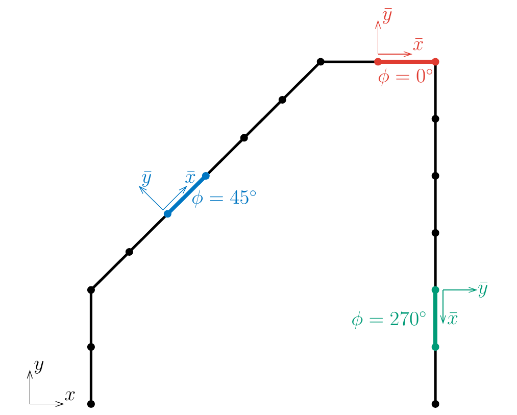
Fig. 4.3 Example of discretization of a 2D frame structure with local coordinate frame indicated for three different elements

For every element in the frame, we can define a local coordinate frame \((\xloc,\yloc)\) that is aligned with the frame element (see Fig. 4.3). Then we have

\[\begin{split} \eps &= \pder{u_\xloc}{\xloc} \\ \gamma &= \pder{u_\yloc}{\xloc}-\theta \\ \kappa &= \pder{\theta}{\xloc} \\ \end{split}\]

The following transformation applies to the displacement vector (and likewise to the force vector):

\[\begin{split} \begin{pmatrix} u_\xloc \\ u_\yloc \end{pmatrix} = \begin{pmatrix} \cos{\phi} & \sin{\phi} \\ -\sin{\phi} & \cos{\phi} \end{pmatrix} \begin{pmatrix} u_x \\ u_y \end{pmatrix} \end{split}\]

As a consequence, we can write

\[\begin{split} \eps &= \cos{\phi}\pder{u_x}{\xloc} + \sin{\phi}\pder{u_y}{\xloc} \\ \gamma &= -\sin{\phi}\pder{u_x}{\xloc} + \cos{\phi}\pder{u_y}{\xloc} - \theta \\ \end{split}\]

This means that with the same definition of \(\ba^e\) as above (in terms of degrees of freedom in global coordinates \(x\) and \(y\)), the strain-displacement matrix becomes:

\[\begin{split} \bB = \begin{bmatrix} \cos{\phi}N_1' & \sin{\phi}N_1' & 0 & \cos{\phi}N_2' & \sin{\phi}N_2' & 0 \\ -\sin{\phi}N_1' & \cos{\phi}N_1' & -N_1 & -\sin{\phi}N_2' & \cos{\phi}N_2' & -N_2 \\ 0 & 0 & N_1' & 0 & 0 & N_2' \\ \end{bmatrix} \end{split}\]

where \(N_i'\) is the derivative of the shape function along the local coordinate \(\xloc\). This is convenient, because shape functions for these elements are initially defined in 1D along the element. For a 2-noded line element with length \(L^e\), the derivatives of the shape functions are given as:

\[ N_1' = -\frac1{L^e} \quad \text{and} \quad N_2' = \frac1{L^e} \]

irrespective of the orientation of the element.

The element stiffness matrix is then defined in exactly the same form as before, except that integration takes place along the element:

\[ \bK^e = \int_{\Omega^e} \bB^T\bD\bB \,d \bar{x} \]

Where \(\Omega^e\) is the domain of the element in local coordinate frame. The exact bounds depend on the choice for how the local coordinate frame is defined. For instance, if \(\bar{x}\) is defined such that it is equal to zero at the first node of the element, the integration will be over \(\bar{x}\in[0,L^e]\).

Contrast with continuum formulations

Firstly, you may notice that in this story there has been no explicit definition for the global stiffness matrix. For 1D problems and continuum problems in 2D or 3D, it can be a useful perspective to consider shape functions as being defined globally and introduce the element-by-element integration and assembly of the global stiffness matrix later on in the derivation. Here, in a case with 1D elements in 2D or 3D space, it would become quite cumbersome to define global shape functions and define global integration over the collection of 1D objects that form the frame. Therefore, we immediately formulate the element matrix here, knowing that this is in the end what is needed in the finite element implementation. Because the degrees of freedom and hence \(\bK^e\) are defined in terms of global coordinate frame, the assembly of the global matrix by putting element matrices in the right position is done with exactly the same procedure as otherwise.

Secondly, we have not used a strong form. For the the extensible beam, the strong form consists of three ODE’s, one independent ODE for the rod plus two coupled ODEs for the beam. For the arbitrarily oriented beam, we have not written strong form equations. The connection between differently oriented elements can be interpreted mechanistically through the concept of element force vectors from Equation (4.73). By assembling the global matrix, a global force vector arises where forces from different connected elements should together be in equilibrium with an external force, or just with one another in absence of any external force on the node. A more formal global derivation for finite elements for space frames is possible with the virtual work equation as starting point instead of the strong form.

Finally, there is also no need for isoparametric mapping. Shape functions and integration scheme are defined in local coordinate \(\bar{x}\). No mapping between \((\bar{x},\bar{y})\) and \((x,y)\) coordinates is needed, only a transformation of vectors: we have discussed this for displacements, and the same transformation is applied implicitly on forces through the \(\phi\)’s in \(\bB^T\) in the element matrix formalation. A choices needs to be made on where \(\bar{x}\) is defined to be zero. A mapping between \(\bar{x}\in[0,L^e]\) and a local coordinate \(\xi\in[-1,1]\) can be introduced but does bring much benefit.