\(\newcommand{\pder}[2]{\frac{\partial #1}{\partial #2}}\) \(\newcommand{\lpder}[2]{\partial #1/\partial #2}\) \(\newcommand{\eps}{\varepsilon}\) \(\newcommand{\beps}{\boldsymbol\varepsilon}\) \(\newcommand{\ba}{\mathbf{a}}\) \(\newcommand{\bff}{\mathbf{f}}\) \(\newcommand{\bu}{\mathbf{u}}\) \(\newcommand{\bzero}{\mathbf{0}}\) \(\newcommand{\bB}{\mathbf{B}}\) \(\newcommand{\bD}{\mathbf{D}}\) \(\newcommand{\bK}{\mathbf{K}}\) \(\newcommand{\bW}{\mathbf{W}}\) \(\newcommand{\bN}{\mathbf{N}}\) \(\newcommand{\bsig}{\boldsymbol\sigma}\) \(\newcommand{\ue}{\mathrm{e}}\) \(\newcommand{\fint}{\mathbf{f}_\mathrm{int}}\)

5.4. Geometrically nonlinear problems

So far in our discussions of the finite element method for applications in solid mechanics, we have dealt with geometrically linear formulations. Deformations, i.e. strain or other strain-like quantities like curvature, have been defined as a linear function of displacements (and, where applicable, rotations). In other words, the kinematic relation was linear. However, this is not always appropriate. Different sources of nonlinearity in kinematic relations can be distinguished. In this introductory section to geometrically nonlinear finite element formulations, the two main ones will be introduced:

• large strains as will be illustrated with a 1D rod

• large displacements (at small strains) as will be illustrated with a rod in 2D space

In finite element literature, the word finite is often used instead of large, so finite strain and finite displacement approaches give rise to geometrically nonlinear finite element formulations.

Rod in 1D: finite strain versus small strain

In a 1D rod element, the strain has been defined as

(5.18)\[ \eps = \pder{u}{x} \]

In a finite element context, where we have \(u(x)=\bN(x)\ba\), the linear dependence on \(\ba\) is apparent in the linear operation

\[ \eps = \bB\ba \]

For a uniform deformation where a rod extends from initial length \(L_0\) to current length \(L\), Equation (5.18) is equivalent to

(5.19)\[ \eps = \frac{L-L_0}{L_0} \]

Again, it is not hard to see that \(L\) is linearly dependent on the axial displacements at both ends of the rod.

However, other strain definitions exist. The strain measure from Equation (5.19) is generally referred to as the engineering strain. An alternative measure is called the true strain:

(5.20)\[ \eps = \ln\left(\frac{L}{L_0}\right) \]

The engineering strain and true strain measures are in fact equivalent for small deformations: Equation (5.19) is the first order Taylor approximation of Equation (5.20) around \(L=L_0\).

For many engineering applications, deformations remains small, if only because many engineering materials cannot withstand large strains: they break at a strain of a few percent. However, even if the material does not deform much, nonlinear strain definitions can be significant. This is the case when rotations are significant for which we need to turn to higher dimensions.

Rod in 2D: finite displacements versus small displacements

Consider the same rod, initially aligned with a global \(x\)-axis, but now in 2D space. The ends of the rod can deform in \(x\) and \(y\) directions. Let’s assume the rod is fixed at the left end (\(u_x(0)=u_y(0)=0\)) and there can be a displacement \(\left(u_x(L),u_y(L)\right)\) at the right end.

We assume the strain in the material remains small, so we adopt the engineering strain definition of Equation (5.19). As long as \(u_y(L)=0\), the engineering strain gives a strain definition that is linear in \(u_x(L)\):

\[ L = L_0 + u_x(L) \quad\Rightarrow\quad \eps = \frac{u_x(L)}{L_0} \]

However, if \(u_x(L)\) and \(u_y(L)\) are both allowed to take nonzero values, we get

\[ L = \sqrt{\left(L_0+u_x(L)\right)^2 + \left(u_y(L)\right)^2} \]

Here, the engineering strain which is linear in \(L\) becomes nonlinear in \(u\) because of the nonlinear relation between \(L\) and \(u\). This nonlinearity exists no matter how big or small \(\eps\) is. Of course, the resulting relation between the strain and the displacements can be linearized under the assumption that displacements are small, but it should be emphasized that this is an additional assumption on top of the small strain assumption.

Geometrically nonlinear frame analysis

Geometric nonlinearity is particularly relevant for slender structures. Cables are one example, where there is tensile action only, but the orientation of the tensile force depends on the orientation of the cable. Frames are another example, where often compressive loading is dominant, which may give rise to buckling. In order to analyze buckling in frames, a geometric nonlinear frame formulation is needed.

Starting point is the 2-node linear frame element introduced earlier as an extensible Timoshenko beam element with arbitrary orientation. The strain vector \(\beps = \left(\eps,\gamma,\kappa\right)^T\) is related to the degrees of freedom \(\ba^\ue =\left(u_{x1}, u_{y1}, \theta_1, u_{x2}, u_{y2}, \theta_2\right)^T\) as

\[ \beps = \bB\ba^\ue \]

with

\[\begin{split} \bB = \frac1{L^\ue } \begin{bmatrix} -\cos{\phi} & -\sin{\phi} & 0 & \cos{\phi} & \sin{\phi} & 0 \\ \sin{\phi} & -\cos{\phi} & -L^\ue N_1 & -\sin{\phi} & \cos{\phi} & -L^\ue N_2 \\ 0 & 0 & -1 & 0 & 0 & 1 \\ \end{bmatrix} \end{split}\]

where \(\phi\) is the angle between the element and the global \(x\)-axis. In geometrically nonlinear analysis, we account for the fact that this angle generally changes when there are nonzero displacements. Note that \(L^\ue\) may also change, but we will work in a small-strain/finite-displacement framework, where the change in \(L^\ue \) will remain small.

Central in our nonlinear solver will be a definition of the nonlinear relation between \(\fint\) and \(\ba\). It should take the form

\[ \fint(\ba) = \int_\Omega \bB^T\bsig\,d\Omega \]

where \(\bsig\) is a function of \(\beps\) which is now a nonlinear function of \(\ba\) and \(\bB\) is defined as the derivative of \(\beps(\ba)\).

We need to start from a definition of strain, for which different alternatives are available. Here, we use the following definition:

(5.21)\[\begin{split} \eps &= \frac{L\cos(\theta-\psi)}{L_0}-1 = \frac{L\left(\cos\theta\cos\psi+\sin\theta\sin\psi\right)}{L_0}-1 \\ \gamma &= \frac{L\sin(\theta-\psi)}{L_0} = \frac{L\left(\cos\theta\sin\psi-\sin\theta\cos\psi\right)}{L_0} \\ \kappa &= \theta' \end{split}\]

where \(\psi\) is the rotation of the beam axis which can be expressed in terms of current and reference coordinates as:

\[\begin{split} \cos\psi &= \frac{\Delta x_0\Delta x+\Delta y_0\Delta y}{LL_0} \\ \sin\psi &= \frac{\Delta x_0\Delta y-\Delta y_0\Delta x}{LL_0} \\ \end{split}\]

using

\[\begin{split} &\Delta x_0 = x_2 - x_1 \\ &\Delta x = x_2+u_{x2}-(x_1+u_{x1}) \\ &\Delta y_0 = y_2 - y_1 \\ &\Delta y = y_2+u_{y2}-(y_1+u_{y1}) \end{split}\]

where \((x_i,y_i)\) are the coordinates of node \(i\) in undeformed state.

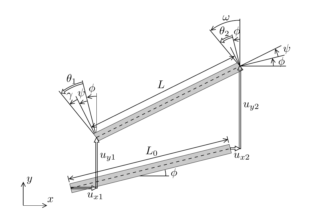
Fig. 5.5 Geometrically nonlinear frame element

The strain definition is derived from the Green-Lagrange strain after selectively applying the assumption of small strain. The current strain definitions are convenient as their derivatives with respect to nodal deformations, which will be collected in the \(\bB\)-matrix, can be expressed in a compact formulation. After a considerable amount of algebra, the following \(\bB\)-matrix is obtained by linearizing the strain measures from Equation (5.21) with respect to the nodal deformations:

(5.22)\[\begin{split} \bB = \pder{\beps}{\ba^\ue} = \frac{1}{L_0} \begin{bmatrix} -\cos\omega & -\sin\omega & L_0N_1\gamma & \cos\omega & \sin\omega & L_0N_2\gamma \\ \sin\omega & -\cos\omega & -L_0N_1(1+\eps) & -\sin\omega & \cos\omega & -L_0N_2(1+\eps) \\ 0 & 0 & -1 & 0 & 0 & 1 \end{bmatrix} \end{split}\]

where \(\omega\) comes from trigonometric considerations and is defined as:

\[ \omega = \phi+\theta \]

The angle \(\omega\) can be considered a measure for the current orientation of the axis. It can readily be observed that for small displacements \(\{\gamma,\eps,\theta\}\ll1\), the \(\bB\)-matrix from the linear formulation is obtained.

Using this definition of \(\beps\) and \(\bB=\lpder{\beps}{\ba^\ue}\), the element forces are defined as:

\[ \fint^\ue = \int_{L_0} \bB^T\bsig\,dx = \int_{L_0} \bB^T\bD\beps\,dx \]

where a linear constitutive law is assumed for the final step. Note that it is no longer possible to compute the element force as the multiplication of the element stiffness matrix with the nodal displacement vector. As opposed to linear analysis, \(\bB\) cannot be used to compute \(\beps\).

In order to linearize the relation between \(\fint^\ue\) and \(\ba^\ue\), we must be aware that both \(\bB\) and \(\beps\) depend on \(\ba^\ue\). Hence, we get:

(5.23)\[ \delta\fint^\ue = \int_{L_0} \bB^T\bD\delta\beps + \delta\bB^T\bsig \,dx \]

When constructing the stiffness matrix, the first term in Equation (5.23) results in a matrix that is very similar to the stiffness matrix from linear analysis. This is called the material stiffness matrix \(\bK^\ue_M\), because it is related to changes in the material. The second term is new. It is called the geometric stiffness matrix \(\bK^\ue_G\) because it is related to changes in the geometry. Therefore, we write:

\[ \bK^\ue = \bK^\ue_M + \bK^\ue_G \]

with

\[ \bK^\ue_M = \int_{L_0}\bB^T\bD\bB\,dx \]

and

\[ \bK^\ue_G = \int_{L_0}\bsig^T\pder{\bB}{\ba^\ue}\,dx \]

For the geometric stiffness matrix we have, in index notation:

\[ K_{G,ij} = \int_{L_0} \sigma_k\pder{B_{ki}}{a_j}\,dx \]

where summation over \(k\) is assumed. It can be observed that the third row of the \(\bB\)-matrix (\(B_{3i}\)) does not depend on the displacements. Therefore there is no contribution from \(M\) to \(\bK_G\). The contributions related to shear force \(V\) and normal force \(N\) can be written separately as:

(5.24)\[ K_G = \int_{L_0} \left(N\bW_N+V\bW_V\right) \,dx \]

with

\[\begin{split} \bW_N = \frac{1}{L_0}\begin{bmatrix} 0 & 0 & N_1\sin\omega & 0 & 0 & N_2\sin\omega \\ 0 & 0 & -N_1\cos\omega & 0 & 0 & -N_2\cos\omega \\ N_1\sin\omega & -N_1\cos\omega & -N_1^2L_0(1+\eps) & -N_1\sin\omega & N_1\cos\omega & -N_1N_2L_0(1+\eps) \\ 0 & 0 & -N_1\sin\omega & 0 & 0 & -N_2\sin\omega \\ 0 & 0 & N_1\cos\omega & 0 & 0 & N_2\cos\omega \\ N_2\sin\omega & -N_2\cos\omega & -N_1N_2L_0(1+\eps) & -N_2\sin\omega & N_2\cos\omega & -N_2^2L_0(1+\eps) \end{bmatrix} \end{split}\]

and

\[\begin{split} \bW_V = \frac{1}{L_0}\begin{bmatrix} 0 & 0 & N_1\cos\omega & 0 & 0 & N_2\cos\omega \\ 0 & 0 & N_1\sin\omega & 0 & 0 & N_2\sin\omega \\ N_1\cos\omega & N_1\sin\omega & -N_1^2L_0\gamma & -N_1\cos\omega & -N_1\sin\omega & -N_1N_2L_0\gamma \\ 0 & 0 & -N_1\cos\omega & 0 & 0 & -N_2\cos\omega \\ 0 & 0 & -N_1\sin\omega & 0 & 0 & -N_2\sin\omega \\ N_2\cos\omega & N_2\sin\omega & -N_1N_2L_0\gamma & -N_2\cos\omega & -N_2\sin\omega & -N_2^2L_0\gamma \\ \end{bmatrix} \end{split}\]

As the numerical stiffness matrix is supposed to be the exact linearization of the numerical force vector, the same integration rule must be chosen for \(\bK_G\) as the one that is used for \(\fint^\ue\). Therefore, the whole element routine can be performed with a single integration point in the middle of the element.

Meaning of \(\bK_M\) and \(\bK_G\)

In the geometrically nonlinear analysis, the product rule of differentiation on \(\fint(\ba)\) gives rise to two terms. The first term, \(\bK_M\), is associated with dependence of \(\bsig\) on \(\ba\): a change in displacements give rise to change in strain and then to a change in stress and eventually to a change in internal forces. Although the \(\bB^T\bD\bB\) expression is the same as in the defintion of the stiffness matrix from linear problems, \(\bK_M\) is also affected by geometric nonlinearity, because the strain-displacement matrix \(\bB\) is the one from Equation (5.22), which also depends on \(\ba\).

The second term \(\bK_G\) represents changes in the geometry at constant stress. A mechanistic interpretation for what it represents can be developed by considering the case of a rotating rod in 2D space. Suppose a rod is strained to a certain amound \(\eps\), there will be a normal force in the rod of magnitude \(N=EA\eps\). The force that needs to be applied at the end of this rod to ensure equilibrium will be equal to \(N\) in magnitude and parallel to the rod orientation. Decomposing this force in \(x\) and \(y\) components will give two values in \(\fint\). Now consider a pure rotation of this rod at constant strain. The elongation \(\eps\) will not change, and neither will the magnitude of the force \(N\). However, the force will change orientation. Then the \(x\) and \(y\) components of this force, which are in \(\fint\) will change.

Geometrically nonlinear continuum mechanics

Linear buckling analysis

With the nonlinear element definitions introduced in the previous sections, different options are possible to analyse buckling behavior. Full nonlinear analysis is possible where the structural response under given load conditions is computed iteratively. In some cases, however, a more elegant solution technique is sufficient to get insight in buckling instability. Under the assumption that deformations are small before instability occurs, it is possible to compute the buckling load from a linear analysis with the geometrically nonlinear element. It will be illustrated in the following what that means.

Instability occurs when there is are multiple equilibrium solutions for a given load. With the material and geometric stiffness matrices \(\bK_M\) and \(\bK_G\), this can be formalized for a given finite element discretization by stating that buckling occurs when:

(5.25)\[ \left[ \bK_M+\lambda \hat{\bK}_G \right] \delta \ba = 0 \quad \text{for any} \quad \delta\ba\neq 0 \]

where \(\hat\bK_G\) is the geometric stiffness matrix for a unit load and \(\lambda\) is the critical load factor. Both \(\bK_M\) and \(\hat\bK_G\) are evaluated in the reference configuration, i.e. with zero deformation. The stresses (\(N\) and \(V\) in (5.24) for a frame problem) used for the evaluation of \(\hat\bK_G\) are those from linear analysis with unit load.

In order to find the critical load factor, the generalized eigenvalue problem in Equation (5.25) must be solved for \(\lambda\). Rows and columns associated with prescribed degrees of freedom must be eliminated before solving the eigenvalue problem to remove rigid body modes. A set of eigenvalues will be found, each of which is the buckling load associated with a certain buckling mode \(\delta\ba\). The lowest eigenvalue gives the buckling load and the corresponding eigenvector is the critical buckling mode.

Linear buckling analysis only works if all loads and prescribed displacements are proportional. It is assumed that the internal stresses from the linear computation with unit load depend linearly on the scalar load factor \(\lambda\). For a case where stress is a combination of a fixed dead-weight and a varying live load, it is not immediately possible to use this method to find the critical load factor for the live load. A more complex decomposition of \(\bK\) into a part that is not affected by the load factor and a part that is a linear function of the load factor would need to be employed.

Implementing linear buckling analysis

Compared to full nonlinear analysis, linear buckling analysis requires slightly different tasks to be implemented. Although the starting point is a nonlinear element formulation, no iterative Newton-Raphson procedure is needed. Instead the generalized eigenvalue problem from Equation (5.25) needs to be solved. This is a mathematical operation that is found in many different applications and for which routines are available. After assembly of \(\bK_G\) and \(\bK_M\) (and removal of rows and columns associated with Dirichlet dofs), scipy can be used to compute critical load factors and buckling modes as:

factors, modes = scipy.linalg.eig(KM, -KG)

where factors contains the solutions for \(\lambda\), of which generally the lowest value is the most relevant output. Additionally, modes contains the eigenvectors \(\delta\ba\) that can be used to visualize buckling modes.

Before the eigenvalue problem is solved, a linear unit load analysis needs to be performed to get the appropriate stress values in \(\hat\bK_G\). For this, the stiffness matrix needs to be evaluated in the undeformed state and \(\hat\ba\) must be evaluated that satisfies

\[ \bK(\bzero)\hat\ba = \hat\bff \]

where \(\hat\bff\) is the unit load vector.

An additional point of attention is that \(\bK_M\) and \(\bK_G\) need to be assembled separately. In a standard linear or nonlinear finite solver, \(\bK\) would be assembled in a single loop over elements where each element puts its own total contribution to \(\bK\). The nonlinear solver then does not need to know the source of nonlinearity. In linear buckling analysis, however, global matrices \(\bK_M\) and \(\hat\bK_G\) must be assembled seperately. Moreover, these must be evaluated at a state that is not entirely consistent in the nonlinear framework, so dedicated routines are needed for this. The \(\bB\)-matrix in \(\bK_M\) must be evaluated at \(\ba=0\). The strain must be computed with that same \(\bB\)-matrix as a first order approximation \(\hat\beps = \bB(\bzero)\hat\ba\), which is not consistent with the nonlinear strain definition, but acceptable under the assumption that displacements are small until instability occurs. After this, we use the linear stress as a consequence of the unit load \(\hat\sigma=\bD\hat\beps\) to evaluate \(\hat\bK_G\).

Hyperelasticity