PyJive workshop: TimoshenkoModel#
import sys
import os
import matplotlib.pyplot as plt
import numpy as np

pyjivepath = '../../../pyjive/'
sys.path.append(pyjivepath)

if not os.path.isfile(pyjivepath + 'utils/proputils.py'):
    print('\n\n**pyjive cannot be found, adapt "pyjivepath" above or move notebook to appropriate folder**\n\n')
    raise Exception('pyjive not found')

from utils import proputils as pu
import main
from names import GlobNames as gn
import contextlib
from urllib.request import urlretrieve

def findfile(fname):
    url = "https://gitlab.tudelft.nl/cm/public/drive/-/raw/main/structural/" + fname + "?inline=false"
    if not os.path.isfile(fname):
        print(f"Downloading {fname}...")
        urlretrieve(url, fname)

findfile("timoshenko.mesh")
findfile("timoshenko.pro")
Cantilever beam example#
Consider the following model of a cantilever beam:
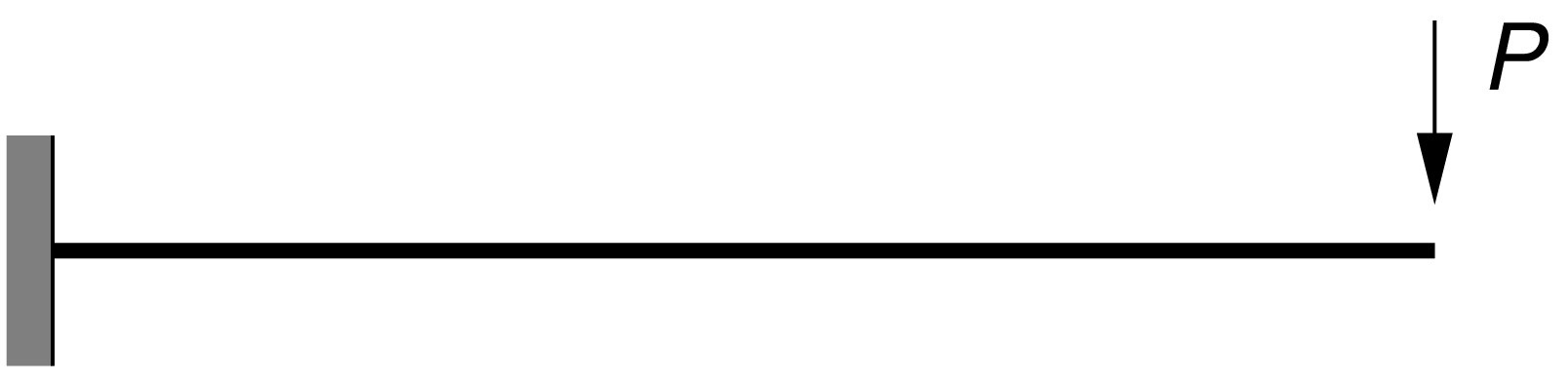
with \(EI=2\cdot 10^4\,\mathrm{Nm}^2\), \(GA_\mathrm{s} = 10^5\,\mathrm{N}\) and \(P=1\,\mathrm{N}\).
The goal here is to examine the response of the finite element solution by considering the vertical displacement \(w\) under the point of application of the load \(P\) and compare it with the analytical solution:
Run the example with input file and mesh file given below and compare your results to the analytical solution.
props = pu.parse_file('timoshenko.pro')
globdat = main.jive(props)
Task 1: Run code block above and inspect results
The solution vector is stored in
globdat[gn.STATE0]. This contains values for all DOFs. Investigate which entry is the displacement at the loaded point and compare its value to the analytical solution.Plot the vertical displacement \(w\) as function of \(x\). Find the values from
globdat[gn.STATE0], construct an array with \(x\)-values (e.g. withnp.linspace), and usematplotlibto create a plot. Can you do the same for rotations?
Mesh-refinement study#
Now we will perform an investigation in how the mesh affects the solution. We can expect the solution to become more accurate when using more elements. Since we have an analytical solution for the end displacement, we can assess how the difference between FEM solution and the exact solution changes when increasing the number of elements. Additionally, we can look at the solution \(w(x)\) for different mesh sizes.
An almost complete code block is provided below.
Task 2: Perform the mesh-refinement study
Compare the end-displacement for different meshes. The comparisons should be made by producing numerical results with 1, 2, 4, 8, 16 and 32 elements and drawing conclusions in terms of accuracy and convergence behavior for the two distinct scenarios below.
Compute the error as the absolute difference between the simulation result and the analytical solution for \(w(L)\). Note that
w_exactis already computed in the code block.After running the cell results in two figures. One shows \(w(x)\) for the different meshes. What is in the other plot?
# function that creates the mesh file
def mesher(L,n):
    dx = L / n
    with open('newmesh.mesh', 'w') as fmesh:
        fmesh.write('nodes (ID, x, [y], [z])\n')
        for i in range(n + 1):
            fmesh.write('%d %f\n' % (i, i * dx))
        fmesh.write('elements (node#1, node#2, [node#3, ...])\n')
        for i in range(n):
            fmesh.write('%d %d\n' % (i, i + 1))
    return globdat

# initializations
number_elements = [1, 2, 4, 8, 16, 32];
L = 10
P = 1
EI = float(props['model']['timoshenko']['EI'])
GA = float(props['model']['timoshenko']['GAs'])
w_exact = P*L**3/3/EI + P*L/GA
props['init']['mesh']['file'] = 'newmesh.mesh'
plt.figure()
errors = []

# loop over different mesh sizes
for ne in number_elements:
    print('\n\nRunning model with',ne,'elements')
    mesher(L,ne)
    globdat = main.jive(props)
    solution = globdat[gn.STATE0]
    plt.plot(np.linspace(0,L,ne+1),solution[ne+1:],label=str(ne) + ' elements')
    err = 1 # evaluate the error here
    errors.append(err)

plt.xlabel('Position [m]')
plt.ylabel('Displacement [m]')
plt.legend()
plt.show()

plt.figure()
plt.loglog(number_elements,errors)
plt.xlabel('Number of elements')
plt.ylabel('Error [m]')
plt.show()
Improve the convergence#
The analysis shown above suffers from shear locking. Recall from the lecture how this can be fixed and try to improve the convergence behavior of the beam.
Task 3: Demonstrate the influence of removing shear locking
Repeat the mesh-refinement study with a modification to your model and compare the accuracy with the results above.
Overwrite one of the entries in
propsto use a locking-free element. Make the change in the notebook rather than intimoshenko.proto keep the ability to rerun previous cells.How is the convergence of the finite element solution to the exact solution affected?
# initializations
plt.figure()
errors_new = []

# loop over different mesh sizes
for ne in number_elements:
    print('\n\nRunning model with',ne,'elements')
    mesher(L,ne)
    globdat = main.jive(props)
    solution = globdat[gn.STATE0]
    plt.plot(np.linspace(0,L,ne+1),solution[ne+1:],label=str(ne) + ' elements')
    err = np.abs(solution[-1]-w_exact)
    errors_new.append(err)

plt.xlabel('Position [m]')
plt.ylabel('Displacement [m]')
plt.legend()
plt.show()

plt.figure()
plt.loglog(number_elements,errors,label='old')
plt.loglog(number_elements,errors_new,label='new')
plt.xlabel('Number of elements')
plt.ylabel('Error [m]')
plt.legend()
plt.show()
Slenderness and shear locking#
Task 4: Repeat with different slenderness
Change \(EI\) and/or \(GA_\mathrm{s}\) in the input file to change the slenderness of the beam. You can check with the analytical solution how big the influence of shear deformation is on the total deflection for any given pair of inputs. Setting \(GA_\mathrm{s}\) very high, you will approach the slender limit. Setting \(EI\) very high will make the problem into a shear-dominated problem.
This notebook has been designed such that the exact solution is updated when you change \(EI\) and \(GA_\mathrm{s}\) in timoshenko.pro. So you can just change the settings and rerun the complete notebook.