Introduction to Numerical methods for ODEs

Let’s assume that we want to find an analytical expression of a function that describes the displacement an object in time, denoted as \( u(t) \). For simplicity, we assume that this object only has one degree of freedom (DOF), e.g. the vertical displacement of the centre of gravity of a floating vessel. We also assume that the object satisfies the equation of motion given by a linear mass-damping-stiffness system:

\[ m\ddot{u}(t)+c\dot{u}(t)+ku(t)=F(t), \]

with \(m\) the mass of the object, \(c\) the damping and \(k\) the stiffness. \( F(t) \) is a time-dependent forcing term. We also provide appropriate initial conditions, in that case

\[ u(0)=0,\quad\dot{u}(0)=\dot{u}_0. \]

In General, and mostly depending on the complexity of the forcing term \( F(t) \), it is difficult to find an analytical expression that is defined at all times, \(u(t)\, ∀ t\in[0,\infty)\), see red blue in the following figure.

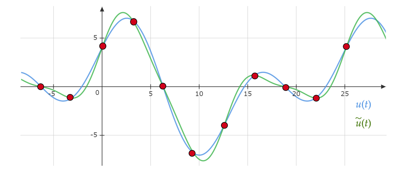
Fig. 6.1 Analytical vs approximated functions

Instead, we might be interested in knowing the value of the function at specific points in time, \(u(t_0),u(t_1),u(t_2),...,u(t_N)\), see red dots in the previous figure. From these set of values, one can reconstruct an approximated function \(\tilde{u}_N(t)\) by, for instance, using a linear interpolation between points (green line in the figure).

For smooth enough functions, \(u(t)\), as we increase the number of evaluation points in time, \(N\), the approximated solution solution \(\tilde{u}_N(t)\) will be closer to \(u(t)\).

Notation

In these notes we will use the following notation, see the figure below:

• \(u_i:=u(t_i)\), the function evaluated at time \(t_i\).

• \(\Delta t_i:=t_i-t_{i-1}\), the time step between two consecutive time steps, \(t_{i-1}\) and \(t_i\). When considering constant time steps, in an interval of time \(t\in[0,T]\) with \(N\) time steps, the time step size will be \(\Delta t=T/N\).

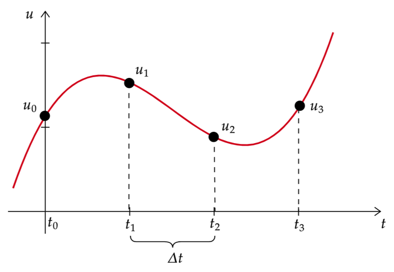
Fig. 6.2 Notation