10.3. Exercise: Visualisation for mechanics and flow simulation#
In this exercise, we are going to make a visualisation that displays both mechanics and flow simulations. On one side, visualisation of a vertical compression of a 2m-long block which is solved with linear elasticity and ideal plasticity. On the other, visualisation of streamlines generated from a 2D simulation of Stokes flow-through on the front face of the block. The data can be downloaded here.
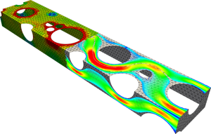
Fig. 10.14 The project from the 4TU-database, exposed at the sixth floor of the CEG building, which we are going to reproduce approximately from the raw simulation data.#
Exercise 1: Visualise the stress distribution#
In this first exercise, we want to visualise the deviatoric stress (von Mises stress) distribution on the deformed block. This is the mechanical part of the problem, simulated in the 3MD_visual_3Dmech.e data file.
Task 1: Download the data, open it in Paraview, and click on Apply.
Solution
Note that we can now see the 2m-long block. Let’s make the visualisation look better and nicer!
Task 2: Show the mesh and the von Mises stress. Make sure the data range is from 0 to 1.
Hint
The mesh can be shown by changing the representation in the Properties Panel to "Surface with Edges". To adjust the data range of the von Mises stress, we can click on "Rescale data to custom range" under Coloring in the Properties Panel and set the values manually.
Solution
Task 3: Pick a desired color map.
Hint
The color map can be changed by clicking on the "Edit color map" button in the Coloring section in the Properties Panel. In this menu, you can choose different preset color maps. Choose the one you like.
Solution
Task 4: Edit the color legend such that the name of the legend is "von Mises" and the legend is located in the top right corner. Make sure it fits by making the legend smaller, changing the font size, and adjusting the color bar thickness.
Hint
The color legend can be edited by clicking on "Edit color bar legend" under Coloring in the Properties Panel. You can drag the legend to the right corner with your mouse and in the menu, you can change the font size and color bar thickness to make sure that it fits perfectly. You can change the format of the text by clicking on the toggle advanced properties (little options sign on the right). Set the "label format" to a notation you like to make sure the legend looks nice.
Solution
Task 5: Use Warp by Vector to visualise the deformations resulting from the applied stress.
Hint
Warp by Vector can be found in the list of common filters.
Solution
Now, we have made a nice visualisation of the mechanical data and the deformation. In the next part of the exercise, we are going to combine the mechanical part with the flow and create an animation.
Exercise 2: Visualise the streamlines and export the animation#
In this part of the exercise, we are going to visualise the flow simulation from the 3MD_2D_flow_front.e data file.
Task 1: Use the calculator to recreate the vector of fluid velocity.
Hint
Using both components vel_X and vel_Y, the formula to input in the calculator is vel_X * iHat + vel_Y * jHat.
Solution
Task 2: Use the transform filter to translate the dataset along the z-axis by the width of the block (4.17).
Hint
In the properties of the transform filter, make sure the translate coordinates are set to: 0, 0, 4.17
Solution
Task 3: Use the stream tracer filter to generate the streamlines of flow.
Hint
Create a line seed at the inlet for the stream tracer below "Line Parameters" in the Properties Panel, across the width of the channel from 0 to 1.94 in the y-axis . Make sure the streamlines remain individually visible by lowering the Resolution parameter if needed.
Solution
Task 4: Use the clip filter to show the streamlines just on one half of the structure.
Hint
Make sure the clip type = box and the length is equal to 11.25 and the width is non zero.
Solution
Task 5: Animate the clipping length to let the streamlines appear over the time of the mechanical simulation.
Hint
Under view, select Time Manager. In this menu we can select Clip1 - ClipType - Length(0) and make sure we add this by clicking on the plus.
Solution
In this exercise, we created a nice looking visualisation for a mechanics and flow problem. Try downloading other examples from the 4TU website to gain more inspiration!