Taylor Series

Taylor Series#

Before going into more details on how to find a numerical approximation, let’s start by refreshing some theory about Taylor series.

the Taylor series of a function is an infinite sum of terms that are expressed in terms of the function’s derivatives at a single point.

That is:

f (x) = \sum_{i = 0}^{\infty} \frac{f^{(i)} (a)}{i!} (x - a)^{i} .

The series is exact for an arbitrary function as long as we include infinite terms in the sum. However, here we are interested on an approximation that includes only the first $r$ terms of the expansion:

f_{r} (x) = \sum_{i = 0}^{r} \frac{f^{(i)} (a)}{i!} (x - a)^{i} \approx f (x) .

Let’s see how this work in a practical example. We consider here the function $f (x) = \sin (x)$ and we want to approximate this function knowing the function value and its derivatives at the point $a = 0$ . Using five terms in the expansion, $r = 5$ , we have that

\begin{array}{r} \begin{aligned} f_{5} (x) & = \sin (0) + x \cos (0) - \frac{x^{2}}{2} \sin (0) - \frac{x^{3}}{6} \cos (0) + \frac{x^{4}}{24} \sin (0) + \frac{x^{5}}{120} \cos (0) \\ = x - \frac{x^{3}}{6} + \frac{x^{5}}{120} . \end{aligned} \end{array}

We now can do a first coding exercise with this example and see how this approximation looks like for different values of $r$ . To do so, we explicitly define the approximated functions.

import numpy as np

n = 200 # Gives smoother functions than standard n=50 linspace
x = np.linspace(-2*np.pi,2*np.pi,n)
a_0 = 0
a = a_0*np.ones(len(x)) # Lower 

def f(x):
  return np.sin(x)
def f0(x):
  return np.sin(a)
def f1(x):
  return f0(x) + (x-a)*np.cos(a)
def f2(x):
  return f1(x) - (x-a)**2/2 * np.sin(a)
def f3(x):
  return f2(x) - (x-a)**3/6 * np.cos(a)
def f4(x):
  return f3(x) + (x-a)**4/24 * np.sin(a)
def f5(x):
  return f4(x) + (x-a)**5/120 * np.cos(a)

Let’s plot all these functions:

import matplotlib.pyplot as plt
%matplotlib inline

plt.plot(x,f(x),label="sin(x)")
plt.plot(x,f0(x),label="f_0(x)",ls=":")
plt.plot(x,f1(x),label="f_1(x)")
plt.plot(x,f2(x),label="f_2(x)",ls=(0, (5, 10)))
plt.plot(x,f3(x),label="f_3(x)")
plt.plot(x,f4(x),label="f_4(x)",ls="dashed")
plt.plot(x,f5(x),label="f_5(x)")

plt.xlabel("x")
plt.ylabel("f(x)"),
plt.xlim((-2*np.pi,2*np.pi))
plt.ylim((-1.5,1.5))
plt.legend();

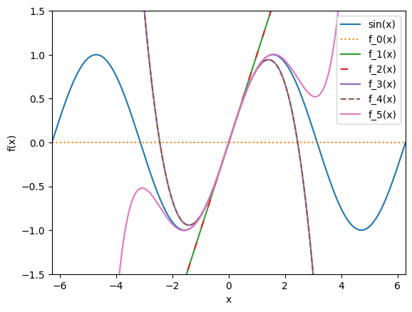
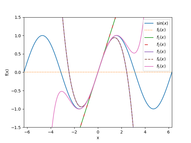
../../_images/d19711ab900beefc017fa3a10d07438a62fe1c4307cf90c893a8fab53dcd2460.png

We see that as we increase the number of terms, the approximation gets closer to the analytical expression. Note also that for this particular example, there is no gain for $r = 2$ and $r = 4$ with respect to $r = 1$ and $r = 3$ . This is caused by the fact that $\sin (a) = 0$ at the approximation point $a = 0$ .

We can go further and evaluate and plot the error of the approximation for different values of $m$ .

e_{m} (x) = | f (x) - f_{m} (x) |, r = 1, . . ., 5

e0 = abs(f(x)-f0(x))
e1 = abs(f(x)-f1(x))
e2 = abs(f(x)-f2(x))
e3 = abs(f(x)-f3(x))
e4 = abs(f(x)-f4(x))
e5 = abs(f(x)-f5(x))

plt.plot(x,np.log10(e0),label="$e_0(x)$",ls=":")
plt.plot(x,np.log10(e1),label="$e_1(x)$")
plt.plot(x,np.log10(e2),label="$e_2(x)$",ls=(0, (5, 10)))
plt.plot(x,np.log10(e3),label="$e_3(x)$")
plt.plot(x,np.log10(e4),label="$e_4(x)$",ls="dashed")
plt.plot(x,np.log10(e5),label="$e_5(x)$")

plt.xlabel("x")
plt.ylabel("log10(e(x))")
plt.xlim((-2*np.pi,2*np.pi))
plt.ylim((10**(-20), 2))
plt.yscale("log")
plt.legend();

plt.savefig("Taylor-series-sin.png")

../../_images/59439820e70802c544a318828a38cddef3dc02fd7030c83ac0c64cf1b8ed519e.png

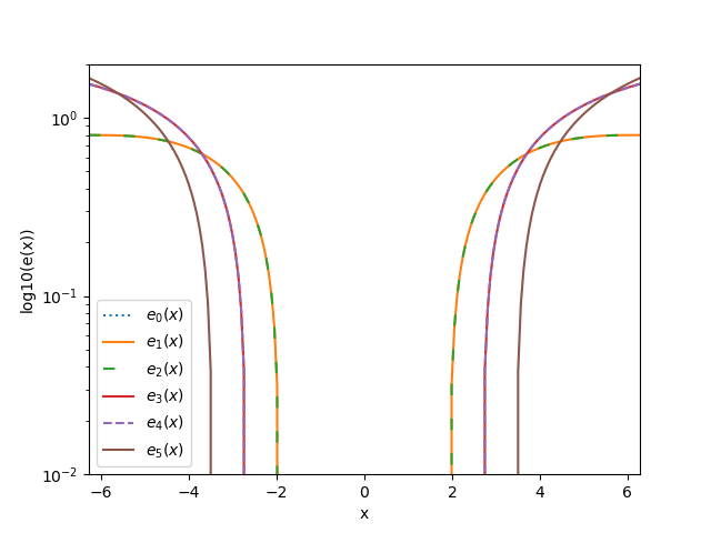
As it is seen in the previous figure, close to the evaluation point $a$ , the approximation error decreases as we increase the number of terms in the expansion.

Examples#

Example 1: Compute the $e^{0.2}$ using Taylor series expansion

We trivially know the value of $f (x) = e^{x}$ for $x = 0$ , and we want to evaluate the value of the function in a point near $x = 0$ . Therefore, we can compute the Taylor series expansion of $e^{x}$

e^{x} \approx e^{0} + x e^{0} + \frac{x^{2}}{2!} e^{0} + \frac{x^{3}}{3!} e^{0} + \frac{x^{4}}{4!} e^{0} \approx 1 + x + \frac{x^{2}}{2} + \frac{x^{3}}{6}

And, therefore, we get:

e^{0.2} \approx 1 + 0.2 + 0.02 + 0.00133 = 1.22133

Example 2: Compute the Taylor expansion of $f (x) = \ln (x)$ around $x = 1$

The Taylor series expansion of $f (x) = \ln (x)$ is given by

f (x) \approx (x - 1) - \frac{1}{2} (x - 1)^{2} + \frac{1}{3} (x - 1)^{3} - \frac{1}{4} (x - 1)^{4}

Exercise#

Compute the Taylor expansion of $f (x) = c o s (x)$ around $x = 0$ . Use the following coding block to compute and plot the true and approximated solution. Use different orders of approximation.

Additional material#

In practise, one can use tools that facilitate the derivation of Taylor series of functions. Primarily these all use the same structure as shown above, however the different functions are created in a loop that more closely resembles the mathematical formulation using factorials. The symbolic basis of the used derivatives is most often done with the Sympy package.

A Similar tool exists for Julia, another scientific programming language that we will look into later in the unit. Then we use the package TaylorSeries.jl, which is a Julia package for Taylor expansions in one or more independent variables.

Here we only focused on functions of one variable, but the same procedure applies for multivariate functions:

The Taylor series expansion for a function of two variables to the second order:

\begin{array}{r} \begin{aligned} f (x, y) \approx f (a, b) & + \frac{\partial f}{\partial x} (a, b) (x - a) + \frac{\partial f}{\partial y} (a, b) (y - b) \\ + \frac{1}{2!} (\frac{\partial^{2} f}{\partial x^{2}} (a, b) (x - a)^{2} + 2 \frac{\partial^{2} f}{\partial x \partial y} (a, b) (x - a) (y - b) + \frac{\partial^{2} f}{\partial y^{2}} (a, b) (y - b)^{2}) \\ + \dots \end{aligned} \end{array}

The Taylor series expansion for a function of two variables to the third order:

\begin{array}{r} \begin{aligned} f (x, y) \approx f (a, b) & + \frac{\partial f}{\partial x} (a, b) (x - a) + \frac{\partial f}{\partial y} (a, b) (y - b) \\ + \frac{1}{2!} (\frac{\partial^{2} f}{\partial x^{2}} (a, b) (x - a)^{2} + 2 \frac{\partial^{2} f}{\partial x \partial y} (a, b) (x - a) (y - b) + \frac{\partial^{2} f}{\partial y^{2}} (a, b) (y - b)^{2}) \\ + \frac{1}{3!} (\frac{\partial^{3} f}{\partial x^{3}} (a, b) (x - a)^{3} + 3 \frac{\partial^{3} f}{\partial x^{2} \partial y} (a, b) (x - a)^{2} (y - b) + 3 \frac{\partial^{3} f}{\partial x \partial y^{2}} (a, b) (x - a) (y - b)^{2} + \frac{\partial^{3} f}{\partial y^{3}} (a, b) (y - b)^{3}) \\ + \dots \end{aligned} \end{array}

Taylor Series

Contents

Taylor Series#

Examples#

Exercise#

Additional material#