Solving the Euler-Bernoulli equation with Continuous/Discontinuos Finite Elements

In this tutorial we will learn how to solve the steady-state Euler-Bernoulli beam equation using a Continuous/Discontinuous Finite Element approximation using Gridap.

This method was introduced by G. Engel and co-authors [1] and has the main advantage that it enables the use of Finite Elements with Lagrange polynomials to solve problems with fourth-order derivatives, which typically require other type of Finite Elements with continuous derivatives.

In addition, in this tutorial we will learn the following Gridap features:

New Gridap features:

• Define distributed loads that depend on the coordinate

• Compute jump and average quantities at the element interfaces

• Operate with vectorial and tensor quantities

• Evaluate the solution at a given point

Problem setting

Let us consider the steady-state Euler-Bernoulli beam equation and associated boundary conditions:

\[\begin{split} \begin{align} \frac{\partial^2 }{\partial x^2}\left(EI \frac{\partial^2 v}{\partial x^2}\right) &= q\qquad&\text{in $\Omega$},\\ v &= v_D\qquad&\text{in $\Gamma_D$},\\ \frac{\partial v}{\partial x} &= \theta_D\qquad&\text{in $\Gamma_D$},\\ EI\frac{\partial^2 v}{\partial x^2} &= M_N\qquad&\text{in $\Gamma_N$},\\ EI\frac{\partial^3 v}{\partial x^3} &= V_N\qquad&\text{in $\Gamma_N$}. \end{align} \end{split}\]

Where \(\Gamma_D\) are the Dirichlet boundaries with prescribed deflection, \(v_D\), and rotation, \(\theta_D\), and \(\Gamma_N\) are the Neumann boundaries with prescribed moment, \(M_N\), and shear, \(V_N\). Note that \(q\) is an external load that can depend on the \(x\)-coordinate.

As an initial setup we will consider the left end as a fixed boundary (\(\Gamma_D\)), \(v_D=0\) and \(\theta_D=0\) and the right end as a free boundary (\(\Gamma_N\)), \(M_N=0\) and \(V_N=0\).

Domain discretization

Here we will follow the steps defined in tutorial 1, feel free to check this tutorial for in-depth description of all the steps. Again, we will use a one-dimensional beam of size \(L=3.0\), discretized using 10 elements.

using Gridap

L = 3
domain = (0,L)
partition = (10,)
model = CartesianDiscreteModel(domain,partition)

We tag the left and right boundaries to apply boundary conditions later on:

labels = get_face_labeling(model)
add_tag_from_tags!(labels,"left",[1])
add_tag_from_tags!(labels,"right",[2])

We can now define the interior and boundary triangulations:

Ω = Triangulation(model)
Γₗ = Boundary(Ω,tags="left")
Γᵣ = Boundary(Ω,tags="right")

In addition, in this tutorial we will see that we need a skeleton triangulation. This is nothing else than the set of interior points where jump conditions will be applied. Note that in a 2D domain the skeleton would be composed by the interior edges of the triangulation, and in a 3D domain by the interior faces of the triangulation.

Λ = Skeleton(Ω)

We can visualize the different triangulations using Paraview as follows:

writevtk(Ω,"Omega")
writevtk(Γₗ,"Gamma_left")
writevtk(Γᵣ,"Gamma_right")
writevtk(Λ,"Lambda")

If we open the VTK files, we can see that we have \(\Omega\), defined by the set of black lines in the following figure, \(\Gamma_l\) defined by the red point, \(\Gamma_r\) defined by the blue point and \(\Lambda\) defined by the set of green points.

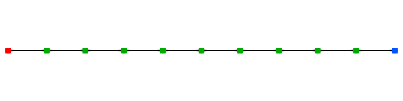
Fig. 4.4 Elements and points of the beam discretization

Finite Element spaces

Traditional Finite Element spaces for fourth-order operators, as the one appearing in the Euler-Bernoulli beam problem, use reference elements with polynomials that satisfy \(C^1\) continuity. This means that both, the unknown and its first derivative are continuous across elements. This can be achieved using, for instance, Hermite polynomials.

However, in this tutorial we will show that Lagrange polynomials can also be used to solve the Euler-Bernoulli beam problem, even though they are only \(C^0\), meaning only the unknown is continuous across elements and not its derivative. Thus, here we follow exactly the same process as the one defined in tutorial 1. The only difference is that here need to use quadratic polynomials at least, since there will appear second derivatives in the weak form.

reffe = ReferenceFE(lagrangian,Float64,2)
Vₕ = TestFESpace(Ω,reffe,dirichlet_tags="left")
Uₕ = TrialFESpace(Vₕ,0.0) 

Note that we can only prescribe strongly the value of the beam deflection \(v_D=0\) on \(\Gamma_l\), because we do not have control of the rotation degree of freedom in the Finite Element space definition.

Discrete form

One of the key steps when deriving the weak form of the Euler-Bernoulli equation is the integration by parts (twice) to go from a fourth-order derivative to the product of two second-order derivatives. This can only be done if the functions are regular enough in the domain where the integration by parts is performed. In a Finite Element context, we integrate by parts at the elemental level and, when using Finite Elements with Lagrange polynomials, there appear terms evaluated at the element boundaries that do not cancel by construction.

Let us see how the final discrete form is defined step by step. We first multiply the strong form by a test function, \(w_h\), and integrate over the full domain \(\Omega\), computing the global integral as a sum of elemental integrals over each element \(K\).

\[ \sum_K\left[\int_K \frac{\partial^2 }{\partial x^2}\left(EI \frac{\partial^2 v}{\partial x^2}\right)w_h\ dK\right] = \sum_K\left[\int_K qw_h\ dK\right]\qquad∀ w_h. \]

Integrating by parts once the term on the left-hand side we have

\[ \sum_{K\in\Omega}\left[-\int_K \frac{\partial }{\partial x}\left(EI \frac{\partial^2 v}{\partial x^2}\right)\frac{\partial w_h}{\partial x}\ dK + \sum_{E\in\partial K}\int_{E} \frac{\partial }{\partial x}\left(EI \frac{\partial^2 v}{\partial x^2}\right) w_h\ dE \right] = \sum_K\left[\int_K qw_h\ dK\right]\qquad∀ w_h. \]

Where \(E\in\partial K\) are the boundaries of an element \(K\), in a one-dimensional element these are the two end points of the element. Note also that in 1D, the integral \(\int_{E} f(x) dE\) is just the evaluation of the function \(f(x)\) at the two boundaries: \(\int_{x_a}^{x_b} f(x) dΓ = f(x_b)-f(x_a)\). We keep the integral notation because is general for arbitrary dimensions and this is how the weak form will be defined in Gridap.

Let us consider two neighboring elements, \(K\) with nodes \(a\) and \(b\), and \(K+1\) with nodes \(b\) and \(c\). We note that when adding the contribution from all the elements, the evaluation of the boundary integrals will lead to the sum of the evaluation of the function from element \(K\) at node \(b\), \(f_K(x_b)\), minus the function evaluated at element \(K+1\) at the same node \(b\), \(f_{K+1}(x_b)\). That is, it will lead to the jump of the function at \(x_b\): \(\newcommand{\jump}[1]{\left[\left|#1\right|\right]}\) \(\newcommand{\mean}[1]{\left\{#1\right\}}\)

\[\text{jump}(f(x_b)) = \jump{f(x_b)} = f_{K+1}(x_b)-f_{K}(x_b).\]

Using the property of \(\jump{a*b} = \jump{a}\mean{b} + \mean{a}\jump{b}\), with \(\text{mean}(a)=\mean{a}=1/2(a_{K}+a_{K+1})\), will lead to the following weak form:

\[ \sum_{K\in\Omega}\left[-\int_K \frac{\partial }{\partial x}\left(EI \frac{\partial^2 v}{\partial x^2}\right)\frac{\partial w_h}{\partial x}\ dK \right] + \sum_{E\in\Lambda}\left[\int_{E} \jump{\frac{\partial }{\partial x}\left(EI \frac{\partial^2 v}{\partial x^2}\right)} \mean{w_h} + \mean{\frac{\partial }{\partial x}\left(EI \frac{\partial^2 v}{\partial x^2}\right)} \jump{w_h}\ dE \right] = \sum_K\left[\int_K qw_h\ dK\right]\qquad∀ w_h. \]

Unless we have a point load or an intermediate support, we want the shear force to be continuous across elements. Therefore, we set the jump of shear force to be zero: \(\jump{\frac{\partial }{\partial x}\left(EI \frac{\partial^2 v}{\partial x^2}\right)} = \jump{V}=0\). In addition, since we use Lagrange polynomials that are continuous, the jump of the test function also cancels, \(\jump{w_h}=0\). Note also that we use the fact that \(w_h=0\) at the Dirichlet boundary and the Neumann boundary condition at the right-end node is: \(V_N=0\). This results in the following form:

\[ \sum_{K\in\Omega}\left[-\int_K \frac{\partial }{\partial x}\left(EI \frac{\partial^2 v}{\partial x^2}\right)\frac{\partial w_h}{\partial x}\ dK \right] = \sum_K\left[\int_K qw_h\ dK\right]\qquad∀ w_h. \]

Now we can integrate by parts again, leading to the following form:

\[ \sum_{K\in\Omega}\left[\int_K EI \frac{\partial^2 v}{\partial x^2}\frac{\partial^2 w_h}{\partial x^2}\ dK \right] + \sum_{E\in\Lambda}\left[\int_{E} - \mean{EI \frac{\partial^2 v}{\partial x^2}} \jump{\frac{\partial w_h}{\partial x}} \ dE \right] + \int_{\Gamma_D} - EI \frac{\partial^2 v}{\partial x^2}\frac{\partial w_h}{\partial x} \ d\Gamma = \sum_K\left[\int_K qw_h\ dK\right]\qquad∀ w_h. \]

Where we have used the fact that moments are continuous across elements: \(\jump{EI \frac{\partial^2 v}{\partial x^2}} = \jump{M}=0\). Here we also used the Neumann boundary condition at the right-end node: \(M_N=0\). Grouping integrals, we can write the discrete problem in a more compact way: find \(v_h\in\mathcal{V}_h\) such that

\[ \int_\Omega EI \frac{\partial^2 v_h}{\partial x^2}\frac{\partial^2 w_h}{\partial x^2}\ dΩ + \int_{\Lambda} - \mean{EI \frac{\partial^2 v_h}{\partial x^2}} \jump{\frac{\partial w_h}{\partial x}} \ d\Lambda + \int_{\Gamma_D} - EI \frac{\partial^2 v}{\partial x^2}\frac{\partial w_h}{\partial x} \ d\Gamma = \int_\Omega qw_h\ d\Omega \qquad∀ w_h\in\mathcal{W}_h. \]

Since we want to enforce continuity of derivatives and we cannot enforce it through the construction of the shape functions, we do it in a weak sense by penalizing the jump of derivatives across elements, \(\jump{\frac{\partial v}{\partial x}}\). We also need to enforce the boundary condition \(\frac{\partial v_h}{\partial x}=0\), which cannot be enforced strongly through the Finite Element space. Therefore, the last step consists on adding additional terms that penalize this jump and the boundary condition for the rotation, see reference [^1] for details. This results in the following weak form:

\[ \int_\Omega EI \frac{\partial^2 v_h}{\partial x^2}\frac{\partial^2 w_h}{\partial x^2}\ dΩ + \int_{\Lambda} \left[- \mean{EI \frac{\partial^2 v_h}{\partial x^2}} \jump{\frac{\partial w_h}{\partial x}} - \mean{EI \frac{\partial^2 w_h}{\partial x^2}} \jump{\frac{\partial v_h}{\partial x}} + \frac{EI\gamma}{h}\jump{\frac{\partial v_h}{\partial x}} \jump{\frac{\partial w_h}{\partial x}}\right]\ d\Lambda + \int_{\Gamma_D} \left[- EI \frac{\partial^2 v_h}{\partial x^2} \frac{\partial w_h}{\partial x} - EI \frac{\partial^2 w_h}{\partial x^2} \frac{\partial v_h}{\partial x} + \frac{EI\gamma}{h}\frac{\partial v_h}{\partial x} \frac{\partial w_h}{\partial x}\right]\ d\Gamma= \int_\Omega qw_h\ d\Omega \qquad∀ w_h\in\mathcal{W}_h. \]

Where \(\gamma>0\) is a constant (we choose \(\gamma=1\) here) and \(h\) is the characteristic element size. In Gridap we will use a more general notation, using vectorial quantities (even if the problem is one-dimensional). Thus, we will use the gradient, \(\nabla(\cdot)\), the laplacian operator, \(\Delta(\cdot)\), and the outer normal to the boundaries \(\mathbf{n}_E\), leading to the following form:

\[ \int_\Omega EI \Delta v_h\Delta w_h\ dΩ + \int_{\Lambda} \left[- \mean{EI \Delta v_h}\jump{\nabla w_h\cdot\mathbf{n}_E} - \mean{EI \Delta w_h}\jump{\nabla v_h\cdot\mathbf{n}_E} + \frac{EI\gamma}{h}\jump{\nabla v_h\cdot\mathbf{n}_E}\jump{\nabla w_h\cdot\mathbf{n}_E}\right] \ d\Lambda + \int_{\Gamma_D} \left[- EI \Delta v_h(\nabla w_h\cdot\mathbf{n}_E) - EI \Delta w_h(\nabla v_h\cdot\mathbf{n}_E) + \frac{EI\gamma}{h}(\nabla v_h\cdot\mathbf{n}_E)(\nabla w_h\cdot\mathbf{n}_E)\right] \ d\Gamma= \int_\Omega qw_h\ d\Omega \qquad∀ w_h\in\mathcal{W}_h. \]

Before coding the weak form, we need to define the integration measures and the normal vectors

dΩ = Measure(Ω,2)
dΛ = Measure(Λ,2)
nΛ = get_normal_vector(Λ)

and the problem parameters, including the forcing term function:

EI = 1.5e7
q(x) = -1.0e3*(L-x[1]) # triangular distributed load

The discrete form is given by the following bilinear and linear forms:

h = L/partition[1]
a(v,w) = ∫( EI*(Δ(v)*Δ(w)) )dΩ +
  ∫( 2*EI/h*((∇(v)⋅nΓₗ)*(∇(w)⋅nΓₗ)) -
    (EI*Δ(v))*(∇(w)⋅nΓₗ) -
    (EI*Δ(w))*(∇(v)⋅nΓₗ) )dΓₗ +
  ∫( EI/h*(jump(∇(v)⋅nΛ)*jump(∇(w)⋅nΛ)) -
    mean(EI*Δ(v))*jump(∇(w)⋅nΛ) -
    mean(EI*Δ(w))*jump(∇(v)⋅nΛ) )dΛ
l(w) = ∫( q*w )dΩ
op = AffineFEOperator(a,l,Uₕ,Vₕ)

Solution and postprocessing

The final step is to compute the solution, which here will be done using the default solver.

vₕ = solve(op)

Once we have the solution we can inspect it using Paraview through the writevtk function. We can also output the gradient of the solution (rotations) directly in the writevtk function.

writevtk(Ω,"EB_solution",cellfields=["v"=>vₕ,"theta"=>∇(vₕ)])

Through Paraview we can visualize the beam deflection and the beam rotation.

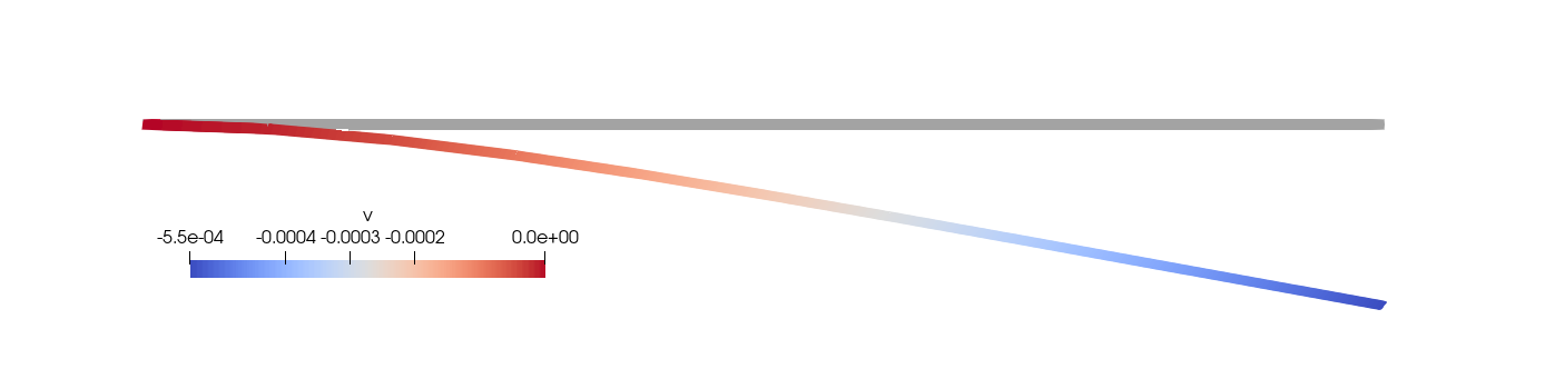
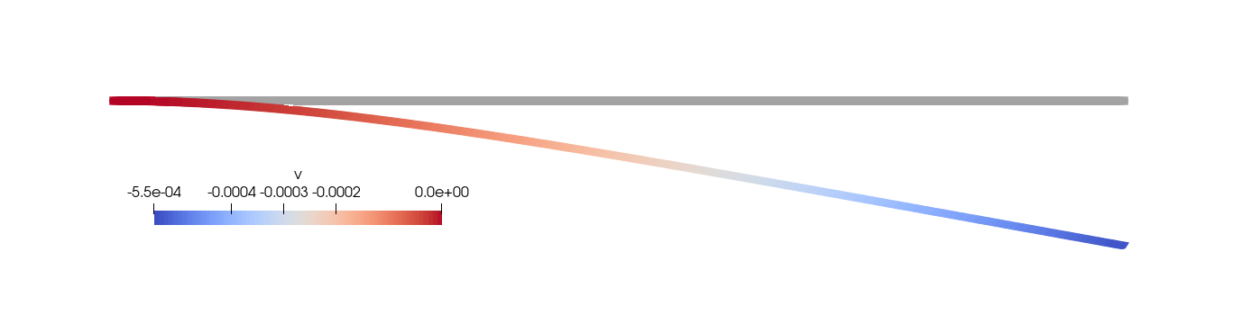
Fig. 4.5 Beam deflection

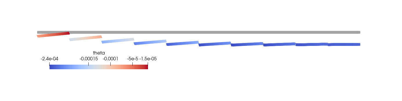
Fig. 4.6 Beam rotations

Note that the rotation is a discontinuous field and it does not satisfy the zero rotation at the left end point. This is because we enforce these conditions in a weak sense. As we refine the mesh, the solution satisfies better these conditions. See below how the deflection and rotations look like when we use a mesh of 100 elements instead of 10.

Fig. 4.7 Beam deflection with 100 elements

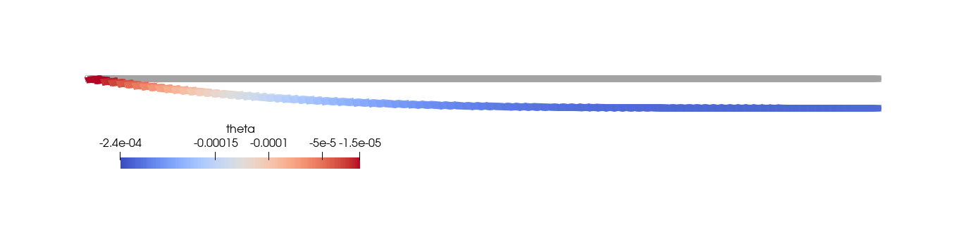
Fig. 4.8 Beam rotations with 100 elements

Sometimes it is useful to evaluate the solution at a given point. This is fairly simple in Gridap, since we just need to evaluate the Finite Element solution sending as argument one or a list of points. A Point is defined sending a tuple with the coordinates. Here we are in a 1D example, so we need to send a tuple with only one entry. If we want to evaluate the deflection at the end of the beam and print it, this will be done as follows:

xₚ = Point((L,))
println(vₕ(xₚ))

Full script

module Euler_Bernoulli
using Gridap

# Discrete model
L = 3.0
domain = (0,L)
partition = (10,)
model = CartesianDiscreteModel(domain,partition)

# Boundary labels
labels = get_face_labeling(model)
add_tag_from_tags!(labels,"left",[1])
add_tag_from_tags!(labels,"right",[2])

# Triangulations
Ω = Triangulation(model)
Γₗ = Boundary(Ω,tags="left")
Γᵣ = Boundary(Ω,tags="right")
Λ = Skeleton(Ω)

# Output triangulations to VTK files
writevtk(Ω,"Omega")
writevtk(Γₗ,"Gamma_left")
writevtk(Γᵣ,"Gamma_right")
writevtk(Λ,"Lambda")

# FE spaces
order = 2
reffe = ReferenceFE(lagrangian,Float64,order)
Vₕ = TestFESpace(Ω,reffe,dirichlet_tags="left")
Uₕ = TrialFESpace(Vₕ,0.0)

# Integration measures and normals
dΩ = Measure(Ω,2*order)
dΓₗ = Measure(Γₗ,1)
dΛ = Measure(Λ,1)
nΓₗ = get_normal_vector(Γₗ)
nΛ = get_normal_vector(Λ)

# Problem parameters
EI = 1.5e7
q(x) = -1.0e3*(L-x[1]) # triangular dustributed load

# Weak form
h = L/partition[1]
a(v,w) = ∫( EI*(Δ(v)*Δ(w)) )dΩ +
  ∫( 2*EI/h*((∇(v)⋅nΓₗ)*(∇(w)⋅nΓₗ)) -
    (EI*Δ(v))*(∇(w)⋅nΓₗ) -
    (EI*Δ(w))*(∇(v)⋅nΓₗ) )dΓₗ +
  ∫( EI/h*(jump(∇(v)⋅nΛ)*jump(∇(w)⋅nΛ)) -
    mean(EI*Δ(v))*jump(∇(w)⋅nΛ) -
    mean(EI*Δ(w))*jump(∇(v)⋅nΛ) )dΛ
l(w) = ∫( q*w )dΩ
op = AffineFEOperator(a,l,Uₕ,Vₕ)

# Solution
vₕ = solve(op)

#Postprocessing
writevtk(Ω,"EB_solution",cellfields=["v"=>vₕ,"theta"=>∇(vₕ)])
xₚ = Point((L,))
println(vₕ(xₚ))

end

References

[1] Engel, G., Garikipati, K., Hughes, T. J. R., Larson, M. G., Mazzei, L., & Taylor, R. L. (2002). Continuous/discontinuous finite element approximations of fourth-order elliptic problems in structural and continuum mechanics with applications to thin beams and plates, and strain gradient elasticity. Computer Methods in Applied Mechanics and Engineering, 191(34), 3669-3750.