7.2. Finite Element implementation

Discrete form

We need to solve for the additional equation terms brought in by the multiphysics couplings. After deriving the strong form of the equation terms into their weak form, they need to be discretised (see Discrete weak form)). The discrete form will as usual correspond to an equation of the type:

(7.1)\[ \mathbf{K} \mathbf{a} = \mathbf{f} \]

With \(\mathbf{K}\) the stiffness matrix, \(\mathbf{a}\) the solution vector and \(\mathbf{f}\) the force vector.

Each variable has to be solved for at every node, which indicates the number of degrees of freedom (DOFs) of the system, characterized by the size of vector \(\mathbf{a}\). Adding additional physical variables to solve for through multiphysics processes will increase the number of DOFs. For a 1D thermo-mechanical problem solved on a mesh of \(X\) nodes, the number of degrees of freedom for the system will be 2\(X\), as we are solving for \(T\) and \(\mathbf{u}\). Since the size of \(\mathbf{a}\) directly correlates to the size of the stiffness matrix we are solving for, multiphysics problems are generally more computationally heavy as they are trying to invert a larger stiffness matrix.

Multiphysics coupling terms, as shown for example in Multiphysics coupling, contribute to the off-diagonal part of the stiffness matrix. We illustrate it below with an example, by deriving the discrete form of the Stokes flow equations. In its strong form, the system of equations is expressed as:

\[\begin{split} \mu \nabla^2 \mathbf{v} -\nabla P = \mathbf{0} \\ \nabla \cdot \mathbf{v} = 0 \end{split}\]

with the first equation being the conservation of momentum with the fluid velocity \(\mathbf{v}\) as the primary variable and the second equation being the conservation of mass with the fluid pressure \(P\) as the primary variable. After introducing \(\mathbf{w^v}\) and \(\mathbf{w^p}\) are the test functions respectively for \(\mathbf{v}\) and \(P\), we can derive the weak form as:

\[\begin{split} \int_\Omega \mu \nabla \mathbf{v} : \nabla \mathbf{w^v} \, d\Omega - \int_\Omega P \, (\nabla \cdot \mathbf{w^v}) \, d\Omega &= 0 \\ \int_\Omega \mathbf{w^p} \, (\nabla \cdot \mathbf{v}) \, d\Omega &= 0 \end{split}\]

After discretising \(\mathbf{v}\) and \(P\) as

(7.2)\[\begin{split} \mathbf{v} \approx \sum_{i=1}^{n}N^\mathbf{v}_{i}v_i \\ \mathbf{p} \approx \sum_{i=1}^{m}N^p_{i}P_i \end{split}\]

where \(n\) are the number of degrees of freedom for \(\mathbf{v}\) and \(m\) for \(P\), the discrete form can be derived as:

\[\begin{split} \mathbf{A} \mathbf{v} - \mathbf{B}^T \mathbf{p} &= \mathbf{0} \\ \mathbf{B} \mathbf{v} &= \mathbf{0} \end{split}\]

where

\[\begin{split} A_{ij} = \int_\Omega \mu \nabla \mathbf{N^v}_i : \nabla \mathbf{N^v}_j \, d\Omega \\ B_{ij} = \int_\Omega N^p_i \, (\nabla \cdot \mathbf{N^v}_j) \, d\Omega \end{split}\]

The system of equations can be rewritten in a matrix form, to retrieve a similar equation as Eq. (7.1) and reveal the stiffness matrix, the solution vector and the force vector.

\[\begin{split} \begin{bmatrix} \mathbf{A} & \textcolor{red}{-\mathbf{B}^T} \\ \textcolor{red}{\mathbf{B}} & \mathbf{0} \end{bmatrix} \begin{bmatrix} \mathbf{v} \\ \mathbf{p} \end{bmatrix} = \begin{bmatrix} \mathbf{0} \\ \mathbf{0} \end{bmatrix} \end{split}\]

In this form, we can observe that the term \(\nabla P\), which is present as a multiphyics coupling in the conservation of momentum, ends up in the off-diagonal of the stiffness matrix. It is similar for the \(\nabla \cdot \mathbf{v}\) term in the conservation of mass.

We note in Eq. (7.2) that each variable can be discretised differently so their test/shape functions will be dependent on the primary variable considered. Below, we explain how the regularisation for the finite element solution of Stokes flow can be implemented using that particular aspect of the multiphysics coupling. We start by explaining what is the problem.

The number of velocity unknowns is determined by the discretisation of the velocity variable. But the number of equations to solve for the velocity unknowns is mostly dependent on the discretisation of the pressure variable because of the \(\nabla \cdot \mathbf{v}\) term in the conservation of mass. If the number of pressure unknowns is greater than the number of velocity unknowns, we have either a dependent or inconsistent system of equations. This is called the Ladyzhenskaya-Babuška-Brezzi (LBB) condition. To regularise the problem we need to increase the number of pressure unknowns so that it never exceeds the number of velocity unknowns. To enforce it, we can increase the order of interpolation of the variable \(\mathbf{v}\), while keeping a lower interpolation order for \(P\). To this end, a special class of elements can be used, the Taylor hood elements, which are illustrated in Fig. 7.1 for a triangular mesh. For more information on that topic, please refer to that document. This trick is only possible because the discretisation between different variables can be independent.

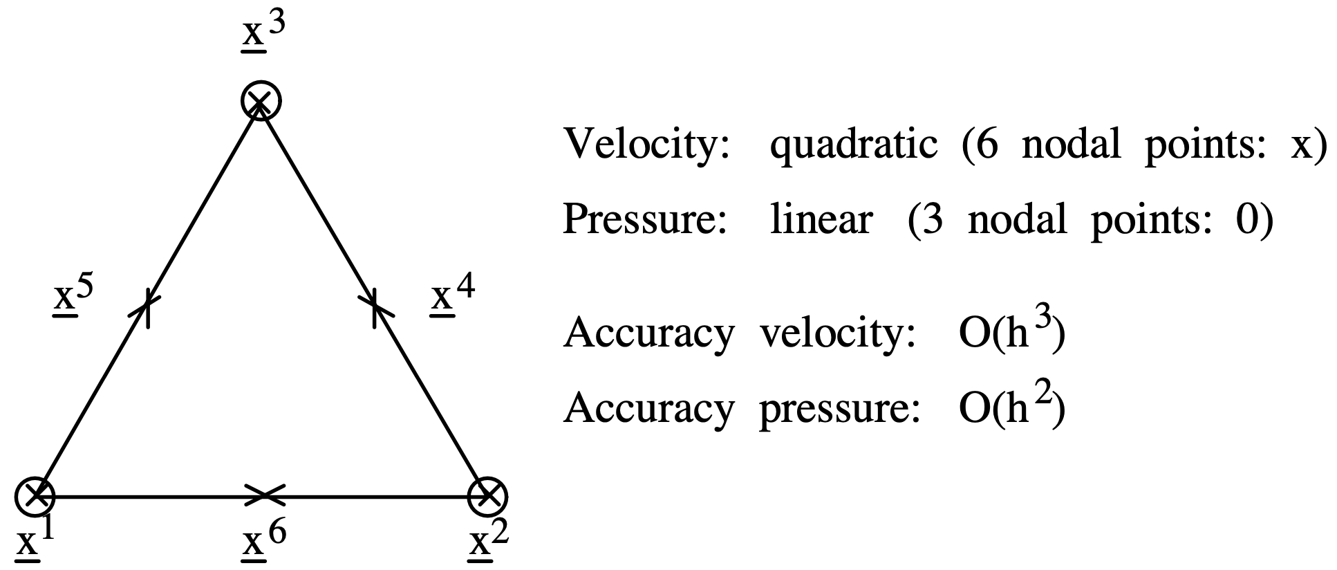
Fig. 7.1 Triangular Taylor-Hood element. Figure from Segal (2023)1.

Boundary conditions

Boundary conditions (BCs) need to apply to each primary variables separately in order to close each governing equation, ensuring a well-posed problem that has a unique and stable solution (see Pyjive workshop on Applying constraints). They are usually described by constant value or constant flow, implemented in Finite Element by respectively Dirichlet or Neumann boundary condition (example in Strong form equation). To give another example for solid mechanics, this corresponds to prescribed displacement (Dirichlet BC of \(\mathbf{u}\)) or prescribed stress (Neumann BC of \(\mathbf{u}\)).

Time discretisation

Physical processes have different time scales. A few examples can be found in Fig. 7.2. Solving for multiphysics means accommodating for all those time scales. The most basic solution is to consider a timestep size aligned with the smallest timescale but that can lead in computational heavy simulations if the timescales have orders of magnitude difference. In that case, instead of solving an implicit coupling, the coupling can remain explicit where the two different physics are solved separately, and the coupled variable is updated at a different frequency adequate to the timescale response.

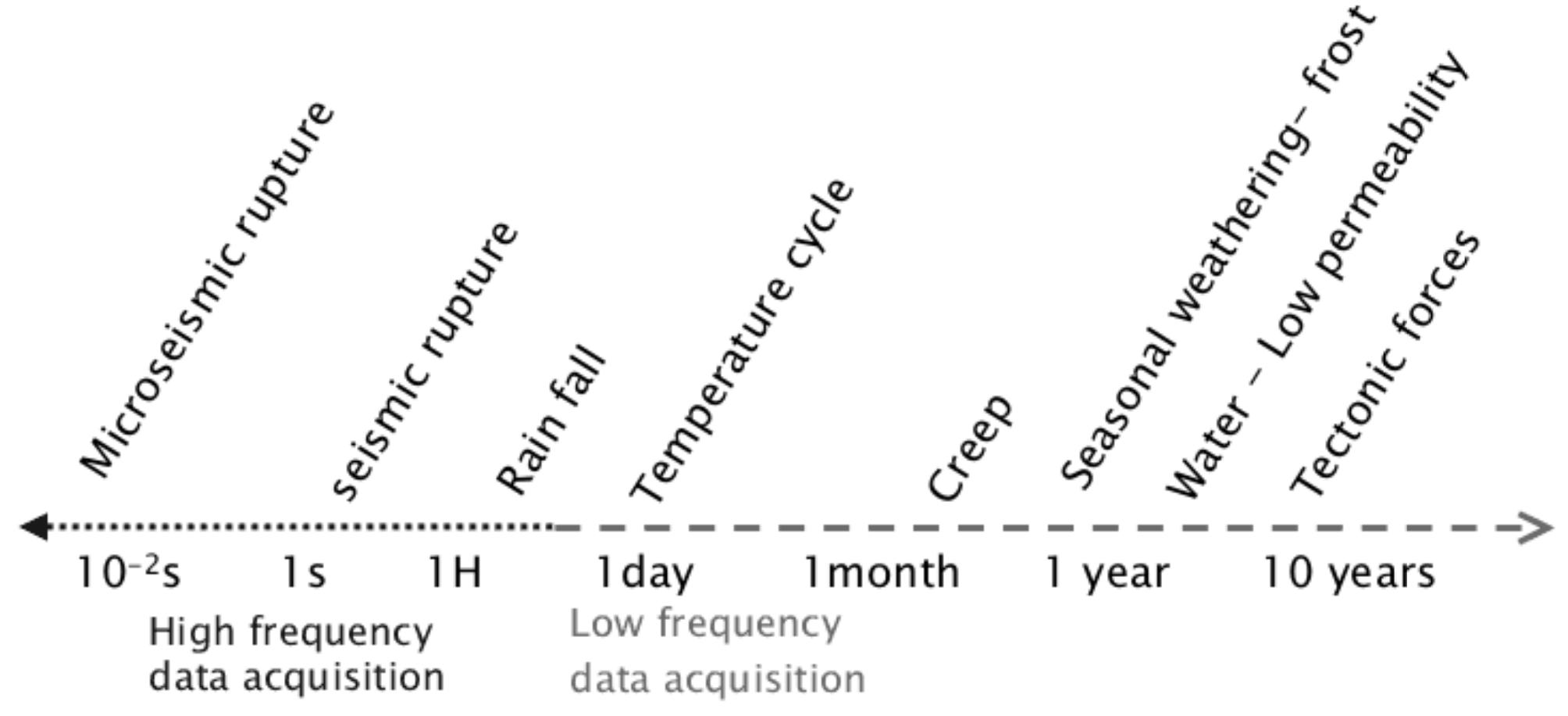
Fig. 7.2 Schematic time scale of some physical processes contributing to the occurrence of a geological instability . Figure from Klein et al. (2008)2

---

1

Segal, A. (2023) Finite element methods for the incompressible Navier-Stokes equations

2

Klein, E. et al. (2008). Global monitoring strategy applied to ground failure hazards. In Proc. of the 10th International Symposium on Landslides and Engineered Slopes.