PyJive workshop: plastic hinges#
This workshop is about analysis of plastic frame problems with pyjive. The main model that is used is the FrameModel. Instead of the NonlinModule, the incremental-iterative procedure is performed with the ArclenModule to allow for capturing post-peak response with proportional loading.
import matplotlib.pyplot as plt
import numpy as np

import contextlib
import os
import sys

pyjivepath = '../../../pyjive/'
sys.path.append(pyjivepath)

if not os.path.isfile(pyjivepath + 'utils/proputils.py'):
    print('\n\n**pyjive cannot be found, adapt "pyjivepath" above or move notebook to appropriate folder**\n\n')
    raise Exception('pyjive not found')

from utils import proputils as pu
import main
from names import GlobNames as gn

%matplotlib widget
from urllib.request import urlretrieve

def findfile(fname):
    url = "https://gitlab.tudelft.nl/cm/public/drive/-/raw/main/plastic-frame/" + fname + "?inline=false"
    if not os.path.isfile(fname):
        print(f"Downloading {fname}...")
        urlretrieve(url, fname)

findfile('beam.pro')
findfile('beam.geom')
findfile('frame.pro')
findfile('frame.geom')
1. Beam with axial and lateral load#
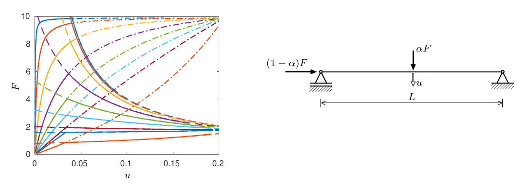
In this notebook we consider the geometrically nonlinear behavior of a simply supported beam with two point loads and a plastic hinge. The ratio between the point loads is controlled by the parameter \(\alpha\).
1.1 Geometrically nonlinear elastic analysis#
Starting point is a geometrically nonlinear elastic analysis, with small \(\alpha\) such that the problem is like a perturbed elastic buckling problem.
plt.close('all')
props = pu.parse_file('beam.pro')
globdat = main.jive(props)

def plotFu(globdat):
    # make a customized force-displacement plot
    Ftot = globdat['loaddisp']['left']['load']['dx'] + globdat['loaddisp']['mid']['load']['dy']
    umid = globdat['loaddisp']['mid']['disp']['dy']
    plt.figure()
    plt.plot(umid,Ftot,marker='.')
    plt.xlabel('u')
    plt.ylabel('F')
    plt.show()

plotFu(globdat)
1.2 Analysis with plastic hinges#
To add plastic hinges, the plastic flag in the FrameModel input is set to True and an additional input parameter is specified, the plastic moment capacity of the cross-section \(M_\mathrm{p}\)
props = pu.parse_file('beam.pro')
props['model']['frame']['plastic'] = 'True'
props['model']['frame']['Mp'] = '0.4'

plt.close('all')
globdat = main.jive(props)
plotFu(globdat)
1.3 Analysis with higher value for \(\alpha\)#
By changing \(\alpha\), the type of response changes. Previously, the solution was that of a buckling problem with material nonlinearity during post-buckling. With \(\alpha=0.5\) it becomes a bending dominated problem.
alpha = 0.5
plt.close('all')
props['model']['neum']['loadIncr'] = str([1-alpha,alpha])
globdat = main.jive(props)
plotFu(globdat)
1.4 Different values of \(\alpha\)#
Finally, the analysis is repeated with a range of different values for \(\alpha\). Note we use contextlib.redirect_stdout here to suppress the output written by pyjive.
# function that runs analysis for given load case
def run_analysis(alpha,props):
    props['model']['neum']['loadIncr'] = str([1-alpha,alpha])
    with contextlib.redirect_stdout(open(os.devnull, "w")):
        globdat = main.jive(props)
    F = globdat['loaddisp']['left']['load']['dx'] + globdat['loaddisp']['mid']['load']['dy']
    u = globdat['loaddisp']['mid']['disp']['dy']
    print('done with analysis with alpha ' + str(alpha))
    return F, u

# switch off frameviewmodule
if 'frameview' in props:
    del props['frameview']

# run analysis for a number of different alphas
plt.close('all')
for alpha in [0.001,0.01,0.02,0.05,0.1,0.2,0.5,1,1.5]:
    F,u = run_analysis(alpha,props)
    plt.plot(u,F)
plt.show()
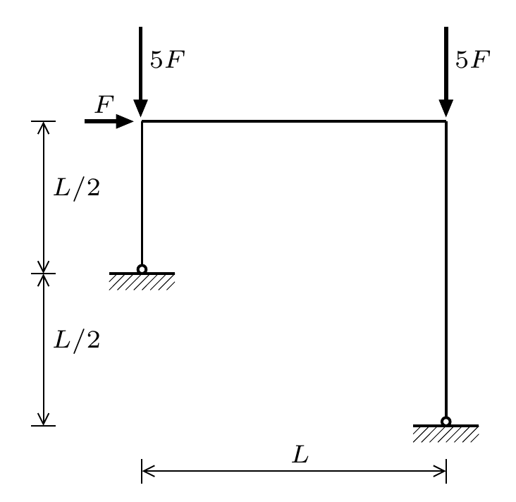
2. Frame with lateral loading#
Secondly, the plastic collapse of a frame is analysed. The geometry visualized below is used, in combination with \(L=2\), \(EI=10\), \(EA=20000\), \(GA=10000\).
2.1 Geometrically nonlinear analysis#
Starting point is geometrically nonlinear elastic analysis. Load-displacement data is stored to allow for a comparison between results from different analyses later on.
props = pu.parse_file('frame.pro')
globdat = main.jive(props)

def getFu(globdat):
    F = globdat['loaddisp']['topleft']['load']['dx']
    u = globdat['loaddisp']['topleft']['disp']['dx']
    return np.vstack((u,F))

FuPlasNL = getFu(globdat)
To further inspect the mechanical response, we can create a new FrameViewModule in the notebook.
fv = globdat[gn.MODULEFACTORY].get_module('FrameView','fv')

props['fv'] = {}
props['fv']['plotStress'] = 'M'
props['fv']['deform'] = '1'
props['fv']['interactive'] = 'True'
props['fv']['plotNeumann'] = 'False'
props['fv']['step0'] = 100

plt.close('all')
fv.init(props, globdat)
status = fv.run(globdat)
fv.shutdown(globdat)
2.2 Geometrically linear version#
The FrameModel has the ability to do geometrically linear analysis as well. This is achieved by setting the subtype to linear. From the immediate convergence and from the shape of the load-displacement curve, it can be observed that the analysis is indeed linear (except for discrete events when the plastic hinges are added). Do you notice the difference in displacements compared to the nonlinear analysis?
plt.close('all')
props = pu.parse_file('frame.pro')
props['model']['frame']['subtype'] = 'linear';
globdat = main.jive(props)

FuPlasLin = getFu(globdat)
A comparison with an analytical solution for the second order rigid-plastic response of this frame is possible. The analytical solution, gives the following relation between force and displacement for the structure after development of the plastic mechanism:
Mp = float(props['model']['frame']['Mp'])
L = 2
uanalytical = np.linspace(0,0.3,100)
Fanalytical = 3*Mp/L*(1-43/3*uanalytical/L)
plt.close('all')
plt.plot(FuPlasNL[0],FuPlasNL[1])
plt.plot(FuPlasLin[0],FuPlasLin[1])
plt.plot(uanalytical,Fanalytical,'--')
plt.plot(uanalytical,Fanalytical[0]*np.ones(uanalytical.shape),'--')
plt.ylim(0,0.7)
plt.show()
It is a bit hard to judge the level of agreement between rigid-plastic and nonlinear finite element solution. This is due to the fact that displacements are already significant when the mechanism develops in the finite element simulation. Therefore, the second order approximation in the rigid-plastic solution is not realistic in the region where the two can be compared.
To check the analytical result, we can let the finite element solution behave more in agreement with the rigid-plastic assumptions. This is done by increasing the stiffnesses.
props = pu.parse_file('frame.pro')
props['model']['frame']['EI'] = '2.e3'
props['model']['frame']['GA'] = '1.e6'
props['model']['frame']['EA'] = '2.e6'
globdat = main.jive(props)

def getFu(globdat):
    F = globdat['loaddisp']['topleft']['load']['dx']
    u = globdat['loaddisp']['topleft']['disp']['dx']
    return np.vstack((u,F))

FuRigPlas = getFu(globdat)
plt.close('all')
plt.plot(FuPlasNL[0],FuPlasNL[1],label='nonlinear elastic/plastic')
plt.plot(FuPlasLin[0],FuPlasLin[1],label='linear elastic/plastic')
plt.plot(FuRigPlas[0],FuRigPlas[1],label='nonlinear rigid/plastic')
plt.plot(uanalytical,Fanalytical,'--',label='analytical 2nd order')
plt.plot(uanalytical,Fanalytical[0]*np.ones(uanalytical.shape),'--',label='analytical 1st order')
plt.xlabel('u')
plt.ylabel('F')
plt.ylim(0,0.7)
plt.legend()
plt.show()
Now, we can see that the analytical second order approximation indeed gives an accurate representation of the initial slope of the force-displacement relation in the plastic mechanism.
The comparison above indicates that the buckling load is of the same order of magnitude as the plastic collapse load, because the maximum load from complete nonlinear analysis including both plasticity and geometric nonlinearity is significantly lower than the plastic collapse load from linear analysis. With linear buckling analysis we can assert whether this is indeed the case. We remove the ArclenModule from the props and add a LinBuckModule
plt.close('all')
props = pu.parse_file('frame.pro')
del props['nonlin']
del props['loaddisp']
del props['graph']

props['model']['neum']['values'] = props['model']['neum']['loadIncr']
props['linbuck'] = {}
props['linbuck']['type'] = 'LinBuck'
globdat = main.jive(props)
Finally, we can check the accuracy of Merchant’s formula for predicting the maximum load \(F_\mathrm{max}\) from the linear plastic collapse load \(F_\mathrm{p}\) and the linear buckling load \(F_\mathrm{b}\) through
Fp = Fanalytical[0]
Fb = globdat[gn.LBFACTORS][0].real
Fmerchant = 1/(1/Fp+1/Fb)
FmaxFEM = max(FuPlasNL[1])
print('Fp        =', Fp)
print('Fb        =', Fb)
print('Fmerchant =', Fmerchant)
print('FmaxFEM   =', FmaxFEM)