Workshop 6: Dynamic string

IMPORTANT: Download the required external functions and put them in the same folder as this notebook
rdeke/ComModHOS_double
rdeke/ComModHOS_double

In this tutorial we will learn how to describe the motion of an oscillating axially deformed string. Here, we will use the FEM to solve a geometrically nonlinear structure subject to gravity loading in a dynamic configuration. The equation of motion of an axially deformed string can be obtained by coupling a string and a rod EOMs, giving the following system of PDEs:

\[ m\ddot{u} -EAu'' = q \]

\[ m \ddot{v} -T v'' = p \]

We follow the general scheme as indicated here:

As usual, we first define the parameters:

import numpy as np
import matplotlib.pyplot as plt
import scipy.integrate as scp

L = 60      # [m] string length
D = 0.75*L  # [m] distance between supports
EA = 1e6    # [Pa] stiffness
m = 1       # [kg] mass
g = 9.81    # [m/s^2] gravity constant

We now define a parameter that will be used as a flag to determine if the string can handle tension only or if it can also handle compression. By default we set it to 1 (tension only). If you want to add the possibility to handle compressions, set it to 0.

TENSION_ONLY = 1

Step 1: discretize the domain

We will use the FEM to solve this problem. Then, we start by discretizing the domain in such a way that the maximum element length \(l_{max}\) is 1 m.

lmax = 5                    # [m] maximum length of each string(wire) element
nElem = int(np.ceil(L/lmax))# [-] number of elements   
lElem = L/nElem             # [m] actual tensionless element size
nNode = nElem + 1           # [-] number of nodes 

We create the nodal coordinates vector and an array with the properties of the element: node connectivity and material properties.

NodeCoord = np.zeros((nNode, 2))
Element = np.zeros((nElem, 5))

for iElem in np.arange(0, nElem):
    NodeLeft = iElem
    NodeRight = iElem + 1
    NodeCoord[NodeRight] = NodeCoord[NodeLeft] + [lElem, 0]
    Element[iElem, :] = [NodeLeft, NodeRight, m, EA, lElem]

Let’s plot the undeformed (horizontal) position of the string, together with the position of the supports

# plot the undeformed wire
plt.figure()
for iElem in np.arange(0, nElem):
    NodeLeft = int(Element[iElem, 0])
    NodeRight = int(Element[iElem, 1])

    plt.plot([NodeCoord[NodeLeft][0], NodeCoord[NodeRight][0]], [NodeCoord[NodeLeft][1], NodeCoord[NodeRight][1]], 'g')
    
# plot the supports
plt.plot(D, 0, 'vr')
plt.axis('equal');

Note that the distance between supports is smaller than the string length. Therefore, the final string position will take a catenary shape between these two points.

Step 2: Dynamic system:

In this tutorial we assume that we have a string that initially is at its static equilibrium position. Then, we add a mass on the left of the string and release the left support.

Step 2.1: Find the initial static position

In order to get the initial string shape, we solve a static problem as done in tutorial 7.1.

nDof = 2*nNode                          # number of DOFs
FreeDof = np.arange(0, nDof)            # free DOFs 
FixedDof = [0,1, -2, -1]                # fixed DOFs
FreeDof = np.delete(FreeDof, FixedDof)  # remove the fixed DOFs from the free DOFs array

# free & fixed array indices
fx = FreeDof[:, np.newaxis]
fy = FreeDof[np.newaxis, :]

SAG = 20                            # Let us assume a big sag - this will assure that all elements
                                    # are under tension, which may be necesary for the convergence
                                    # of the solver
s = np.array([i[0] for i in NodeCoord])
x = D*(s/L)
y = -4*SAG*((x/D)-(x/D)**2)
u = np.zeros((nDof))
u[0:nDof+1:2] = x - np.array([i[0] for i in NodeCoord])
u[1:nDof+1:2] = y - np.array([i[1] for i in NodeCoord])
# The displacement of the node corresponds to the actual position minus the initial position
# Remember that we use a Global Coordinate System (GCS) here.

Pext = np.zeros((nDof))
for iElem in np.arange(0, nElem):
    NodeLeft = int(Element[iElem, 0])
    NodeRight = int(Element[iElem, 1])
    DofsLeft = 2*NodeLeft 
    DofsRight = 2*NodeRight
    l0 = Element[iElem, 4]
    m = Element[iElem, 2]
    Pelem = -g*l0*m/2           # Half weight to each node
    Pext[DofsLeft + 1] += Pelem
    Pext[DofsRight + 1] += Pelem

from StringForcesAndStiffness import StringForcesAndStiffness
# Convergence parameters
CONV = 0
PLOT = False
kIter = 0
nMaxIter = 100
TENSION = np.zeros((nElem))

while CONV == 0:
    kIter += 1
    # Check stability - define a number of maximum iterations. If solution
    # hasn't converged, check what is going wrong (if something).
    if kIter > nMaxIter:
        break
    
    # Assemble vector with internal forces and stiffnes matrix
    K = np.zeros((nDof*nDof)) 
    Fi = np.zeros((nDof))
    for iElem in np.arange(0, nElem):
        NodeLeft = int(Element[iElem, 0])
        NodeRight = int(Element[iElem, 1])
        DofsLeft = 2*NodeLeft 
        DofsRight = 2*NodeRight
        l0 = Element[iElem, 4]
        EA = Element[iElem, 3]
        NodePos = ([NodeCoord[NodeLeft][0] + u[DofsLeft], NodeCoord[NodeRight][0] + u[DofsRight]], 
                    [NodeCoord[NodeLeft][1] + u[DofsLeft + 1], NodeCoord[NodeRight][1] + u[DofsRight + 1]])
        Fi_elem, K_elem, Tension, WARN = StringForcesAndStiffness(NodePos, EA, l0, TENSION_ONLY)
        TENSION[iElem] = Tension
        
        Fi[DofsLeft:DofsLeft + 2] += Fi_elem[0]
        Fi[DofsRight:DofsRight + 2] += Fi_elem[1]

        # Assemble the matrices at the correct place
            # Get the degrees of freedom that correspond to each node
        Dofs_Left = 2*(NodeLeft) + np.arange(0, 2)
        Dofs_Right = 2*(NodeRight) + np.arange(0, 2)
        nodes = np.append(Dofs_Left , Dofs_Right)
        for i in np.arange(0, 4):
            for j in np.arange(0, 4):
                ij = nodes[i] + nodes[j]*nDof
                K[ij] = K[ij] + K_elem[i, j]

    K = K.reshape((nDof, nDof))

    # Calculate residual forces
    R = Pext - Fi

    # Check for convergence
    if np.linalg.norm(R[FreeDof])/np.linalg.norm(Pext[FreeDof]) < 1e-3:
        CONV = 1

    # Calculate increment of displacements
    du = np.zeros((nDof))
    du[FreeDof] = np.linalg.solve(K[fx, fy], R[FreeDof])

    # Apply archlength to help with convergence
    Scale = np.min(np.append(np.array([1]), lElem/np.max(np.abs(du))))
    du = du*Scale   # Enforce that each node does not displace
                    # more (at each iteration) than the length
                    # of the elements

    # Update displacement of nodes
    u += du

    # plot the updated configuration
    if PLOT:
        for iElem in np.arange(0, nElem):
            NodeLeft = int(Element[iElem, 0])
            NodeRight = int(Element[iElem, 1])
            DofsLeft = 2*NodeLeft 
            DofsRight = 2*NodeRight
            plt.plot([NodeCoord[NodeLeft][0] + u[DofsLeft], NodeCoord[NodeRight][0] + u[DofsRight]], 
                        [NodeCoord[NodeLeft][1] + u[DofsLeft + 1], NodeCoord[NodeRight][1] + u[DofsRight + 1]], '-ok')
            
        # plot the supports
        plt.plot([0, D], [0, 0], 'vr')
        plt.axis('equal')
        plt.xlabel("x [m]")
        plt.ylabel("y [m]")
        plt.title("Iteration: "+str(kIter))
        plt.pause(0.05)

if CONV == 1:
    for iElem in np.arange(0, nElem):
            NodeLeft = int(Element[iElem, 0])
            NodeRight = int(Element[iElem, 1])
            DofsLeft = 2*NodeLeft 
            DofsRight = 2*NodeRight
            plt.plot([NodeCoord[NodeLeft][0] + u[DofsLeft], NodeCoord[NodeRight][0] + u[DofsRight]], 
                        [NodeCoord[NodeLeft][1] + u[DofsLeft + 1], NodeCoord[NodeRight][1] + u[DofsRight + 1]], '-ok')
            
    # plot the supports
    plt.plot(D, 0, 'vr')
    plt.axis('equal')
    plt.xlabel("x [m]")
    plt.ylabel("y [m]")
    plt.title("Converged solution at iteration: "+str(kIter))
else:
    print("Solution did not converge")

---------------------------------------------------------------------------
ModuleNotFoundError                       Traceback (most recent call last)
Cell In[6], line 34
     31     Pext[DofsLeft + 1] += Pelem
     32     Pext[DofsRight + 1] += Pelem
---> 34 from StringForcesAndStiffness import StringForcesAndStiffness
     35 # Convergence parameters
     36 CONV = 0

ModuleNotFoundError: No module named 'StringForcesAndStiffness'

Step 2.2: solve the dynamic problem

First, we define the mass on the left node and some damping.

Mass = 100
C = 0.001*EA # just some damping

The external force will be the same as the one used to find the initial position, so here we only need to compute the mass matrix.

M = np.zeros((nDof*nDof))
M[0] = Mass                         # Add mass at the left node
M[nDof + 1] = Mass                  # Add mass at the left node
Pext[1] = Pext[1] - Mass*g          # Add weight to the left node
for iElem in np.arange(0, nElem):
        NodeLeft = int(Element[iElem, 0])
        NodeRight = int(Element[iElem, 1])
        DofsLeft = 2*NodeLeft 
        DofsRight = 2*NodeRight
        l0 = Element[iElem, 4]
        EA = Element[iElem, 3]
        M_elem = m*l0/6*np.array([[2, 0, 1, 0], 
                                    [0, 2, 0, 1], 
                                    [1, 0, 2, 0], 
                                    [0, 1, 0, 2]])
        # Assemble the matrices at the correct place
        # Get the degrees of freedom that correspond to each node
        Dofs_Left = 2*(NodeLeft) + np.arange(0, 2)
        Dofs_Right = 2*(NodeRight) + np.arange(0, 2)
        nodes = np.append(Dofs_Left , Dofs_Right)
        for i in np.arange(0, 4):
            for j in np.arange(0, 4):
                ij = nodes[i] + nodes[j]*nDof
                M[ij] = M[ij] + M_elem[i, j]
M = M.reshape((nDof, nDof))

We define the fixed and free DOFs of the system.

# Release the left support
nDof = 2*nNode                          # number of DOFs
FreeDof = np.arange(0, nDof)            # free DOFs 
FixedDof = [-2, -1]                     # fixed DOFs
FreeDof = np.delete(FreeDof, FixedDof)  # remove the fixed DOFs from the free DOFs array

# free & fixed array indices
fx = FreeDof[:, np.newaxis]
fy = FreeDof[np.newaxis, :]

Now, we have all we need to perform the time integration. We initialize the state vector with zero initial velocities. To solve the ODE we use the solve_ivp function, calling the ACCELERATIONS function as an ode function. You can find the definition of this function below.

Auxiliar function:

The ACCELERATIONS function computes the accelerations based on the equation:

\[ \boldsymbol{M} \ddot{\boldsymbol{u}}_{n+1} = \boldsymbol{F}_{ext} - \boldsymbol{F}_{int}(\boldsymbol{u}_n, \dot{\boldsymbol{u}}_n) \]

from StringDynamicForces import StringDynamicForces
def ACCELERATIONS(t, U, NodeCoord, Element, FreeDof, C, M, Pext, TENSION_ONLY):
    nDof = len(U)
    u = U[:nDof//2]
    v = U[nDof//2:]

    # free & fixed array indices
    fx = FreeDof[:, np.newaxis]
    fy = FreeDof[np.newaxis, :]

    # Calculate internal forces
    FintDyn = np.zeros((nDof))
    for iElem in np.arange(0, len(Element)):
        NodeLeft = int(Element[iElem, 0])
        NodeRight = int(Element[iElem, 1])
        DofsLeft = 2*NodeLeft 
        DofsRight = 2*NodeRight
        l0 = Element[iElem, 4]
        EA = Element[iElem, 3]
        NodePos = ([NodeCoord[NodeLeft][0] + u[DofsLeft], NodeCoord[NodeRight][0] + u[DofsRight]], 
            [NodeCoord[NodeLeft][1] + u[DofsLeft + 1], NodeCoord[NodeRight][1] + u[DofsRight + 1]])
        NodeVel = ([v[DofsLeft], v[DofsRight]], 
                    [v[DofsLeft + 1], v[DofsRight + 1]])
        Fint = StringDynamicForces(NodePos, NodeVel, EA, C, l0)
        FintDyn[DofsLeft:DofsLeft + 2] += Fint[0]
        FintDyn[DofsRight:DofsRight + 2] += Fint[1]

    # Calculate the new acceleration
    a = np.zeros((nDof//2))
    a[FreeDof] = np.linalg.solve(M[fx, fy], (Pext[FreeDof]-FintDyn[FreeDof]))
    
    # Store the derivative of phase
    dU = np.append(v, a)
    #print("Time = "+str(t)+" s")
    return dU

v = u*0
U0 = np.append(u, v)
dt = 0.1
Tend = 10
tspan = np.arange(0, Tend, dt)

def odefun(t, U):
    # print(t) # Can add to follow progress - may take a few minutes
    return ACCELERATIONS(t, U, NodeCoord, Element, FreeDof, C, M, Pext, TENSION_ONLY)

sol = scp.solve_ivp(fun=odefun, t_span=[tspan[0], tspan[-1]], y0=U0, t_eval=tspan)  

Once we have the solution, we can plot the evolution of the string.

%matplotlib inline
import time
from IPython import display

for iT in np.arange(0, len(sol.t)):
    try: 
        u = sol.y[:nDof, iT]
        for iElem in np.arange(0, nElem):
            NodeLeft = int(Element[iElem, 0])
            NodeRight = int(Element[iElem, 1])
            DofsLeft = 2*NodeLeft 
            DofsRight = 2*NodeRight
            plt.plot([NodeCoord[NodeLeft][0] + u[DofsLeft], NodeCoord[NodeRight][0] + u[DofsRight]], 
                        [NodeCoord[NodeLeft][1] + u[DofsLeft + 1], NodeCoord[NodeRight][1] + u[DofsRight + 1]], '-ok')
        # plot the supports
        plt.plot(D, 0, 'vr')     
        plt.axis('equal')
        plt.xlabel("x [m]")
        plt.ylabel("y [m]")
        plt.savefig(f".././images/Module7/w7_t2_gif/shot{iT}.png")
        display.display(plt.gcf())
        display.clear_output(wait=True)
        plt.clf()
        time.sleep(0.01)
    except KeyboardInterrupt:
        break

u = sol.y[:nDof, -1]
for iElem in np.arange(0, nElem):
    NodeLeft = int(Element[iElem, 0])
    NodeRight = int(Element[iElem, 1])
    DofsLeft = 2*NodeLeft 
    DofsRight = 2*NodeRight
    plt.plot([NodeCoord[NodeLeft][0] + u[DofsLeft], NodeCoord[NodeRight][0] + u[DofsRight]], 
                [NodeCoord[NodeLeft][1] + u[DofsLeft + 1], NodeCoord[NodeRight][1] + u[DofsRight + 1]], '-ok')
# plot the supports
plt.plot(D, 0, 'vr') 
plt.axis('equal')
plt.xlabel("x [m]")
plt.ylabel("y [m]");

Now displaying the animated plots, gif conversion via https://ezgif.com/jpg-to-gif.

Exercise

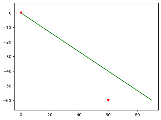
Determine the mooring configuration of a floating wind turbine attached to two cables of different length:

\[L_{left}=100\]

\[L_{right}=90\]

The anchors are positioned at \([-50,-60]\) and \([60,-60]\). The floating wind turbine is at \([0,0]\). Assume for now that the anchor line can go below the seabed. The line properties (Weights, stiffness, ..). However, now the turbine is moving horizontally in the following manner (although unrealistic in the real world): $\( u(t) = 5 \cos(2 t) \)$

A simple visualization is added below (adapted from here).

## Right side
# (The idea for te left side is the same, but with D = 50 and then mirorring the final result)

# Step 1: discretize the domain

L = 90     # [m] string length
D = 60      # [m] distance between supports
H = 60      # [m] water depth
EA = 1e6    # [Pa] stiffness
m = 1       # [kg/m] mass per length of line
g = 9.81    # [m/s^2] gravity constant

lmax = 5                    # [m] maximum length of each string(wire) element
nElem = int(np.ceil(L/lmax))# [-] number of elements   
lElem = L/nElem             # [m] actual tensionless element size
nNode = nElem + 1           # [-] number of nodes 

NodeCoord = np.zeros((nNode, 2))
Element = np.zeros((nElem, 5))

for iElem in np.arange(0, nElem):
    NodeLeft = iElem
    NodeRight = iElem + 1
    NodeCoord[NodeRight] = NodeCoord[NodeLeft] + [lElem, -H/L*lElem]
    Element[iElem, :] = [NodeLeft, NodeRight, m, EA, lElem]
    
# plot the undeformed wire
plt.figure()
for iElem in np.arange(0, nElem):
    NodeLeft = int(Element[iElem, 0])
    NodeRight = int(Element[iElem, 1])

    plt.plot([NodeCoord[NodeLeft][0], NodeCoord[NodeRight][0]], [NodeCoord[NodeLeft][1], NodeCoord[NodeRight][1]], 'g')
    
# plot the supports
plt.plot([0, D], [0, -H], 'vr')
plt.axis('equal');

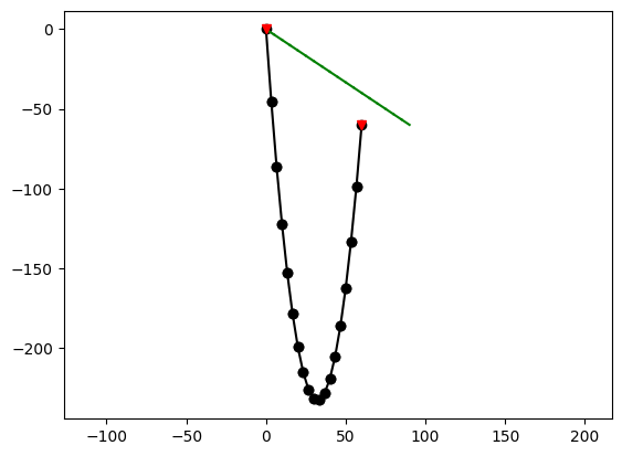
# Step 2: compute initial configuration
# Hint: What estimate for the sag would you use?

nDof = 2*nNode                          # number of DOFs
FreeDof = np.arange(0, nDof)            # free DOFs 
FixedDof = [0,1, -2, -1]                # fixed DOFs
FreeDof = np.delete(FreeDof, FixedDof)  # remove the fixed DOFs from the free DOFs array

# free & fixed array indices
fx = FreeDof[:, np.newaxis]
fy = FreeDof[np.newaxis, :]

SAG = 202
s = np.array([i[0] for i in NodeCoord])
x = D*(s/L)
y = -H*(s/L)-4*SAG*((x/D)-(x/D)**2)
u = np.zeros((nDof))
u[0:nDof+1:2] = x - np.array([i[0] for i in NodeCoord])
u[1:nDof+1:2] = y - np.array([i[1] for i in NodeCoord])
# The displacement of the node corresponds to the actual position minus the initial position
# Remember that we use a Global Coordinate System (GCS) here.

# plot the initial guess
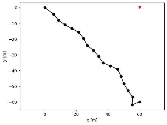
plt.figure()
for iElem in np.arange(0, nElem):
    NodeLeft = int(Element[iElem, 0])
    NodeRight = int(Element[iElem, 1])
    DofsLeft = 2*NodeLeft 
    DofsRight = 2*NodeRight
    plt.plot([NodeCoord[NodeLeft][0] + u[DofsLeft], NodeCoord[NodeRight][0] + u[DofsRight]], 
                [NodeCoord[NodeLeft][1] + u[DofsLeft + 1], NodeCoord[NodeRight][1] + u[DofsRight + 1]], '-ok')
    plt.plot([NodeCoord[NodeLeft][0], NodeCoord[NodeRight][0]], [NodeCoord[NodeLeft][1], NodeCoord[NodeRight][1]], 'g')
    
# plot the supports
plt.plot([0, D], [0, -H], 'vr')
plt.axis('equal');

Pext = np.zeros((nDof))
for iElem in np.arange(0, nElem):
    NodeLeft = int(Element[iElem, 0])
    NodeRight = int(Element[iElem, 1])
    DofsLeft = 2*NodeLeft 
    DofsRight = 2*NodeRight
    l0 = Element[iElem, 4]
    m = Element[iElem, 2]
    Pelem = -g*l0*m/2           # Half weight to each node
    Pext[DofsLeft + 1] += Pelem
    Pext[DofsRight + 1] += Pelem

from StringForcesAndStiffness import StringForcesAndStiffness
# Convergence parameters
CONV = 0
PLOT = False
kIter = 0
nMaxIter = 100
TENSION = np.zeros((nElem))

while CONV == 0:
    kIter += 1
    # Check stability - define a number of maximum iterations. If solution
    # hasn't converged, check what is going wrong (if something).
    if kIter > nMaxIter:
        break
    
    # Assemble vector with internal forces and stiffnes matrix
    K = np.zeros((nDof*nDof)) 
    Fi = np.zeros((nDof))
    for iElem in np.arange(0, nElem):
        NodeLeft = int(Element[iElem, 0])
        NodeRight = int(Element[iElem, 1])
        DofsLeft = 2*NodeLeft 
        DofsRight = 2*NodeRight
        l0 = Element[iElem, 4]
        EA = Element[iElem, 3]
        NodePos = ([NodeCoord[NodeLeft][0] + u[DofsLeft], NodeCoord[NodeRight][0] + u[DofsRight]], 
                    [NodeCoord[NodeLeft][1] + u[DofsLeft + 1], NodeCoord[NodeRight][1] + u[DofsRight + 1]])
        Fi_elem, K_elem, Tension, WARN = StringForcesAndStiffness(NodePos, EA, l0, TENSION_ONLY)
        TENSION[iElem] = Tension
        
        Fi[DofsLeft:DofsLeft + 2] += Fi_elem[0]
        Fi[DofsRight:DofsRight + 2] += Fi_elem[1]

        # Assemble the matrices at the correct place
            # Get the degrees of freedom that correspond to each node
        Dofs_Left = 2*(NodeLeft) + np.arange(0, 2)
        Dofs_Right = 2*(NodeRight) + np.arange(0, 2)
        nodes = np.append(Dofs_Left , Dofs_Right)
        for i in np.arange(0, 4):
            for j in np.arange(0, 4):
                ij = nodes[i] + nodes[j]*nDof
                K[ij] = K[ij] + K_elem[i, j]

    K = K.reshape((nDof, nDof))

    # Calculate residual forces
    R = Pext - Fi

    # Check for convergence
    if np.linalg.norm(R[FreeDof])/np.linalg.norm(Pext[FreeDof]) < 1e-3:
        CONV = 1

    # Calculate increment of displacements
    du = np.zeros((nDof))
    du[FreeDof] = np.linalg.solve(K[fx, fy], R[FreeDof])

    # Apply archlength to help with convergence
    Scale = np.min(np.append(np.array([1]), lElem/np.max(np.abs(du))))
    du = du*Scale   # Enforce that each node does not displace
                    # more (at each iteration) than the length
                    # of the elements

    # Update displacement of nodes
    u += du

    # plot the updated configuration
    if PLOT:
        for iElem in np.arange(0, nElem):
            NodeLeft = int(Element[iElem, 0])
            NodeRight = int(Element[iElem, 1])
            DofsLeft = 2*NodeLeft 
            DofsRight = 2*NodeRight
            plt.plot([NodeCoord[NodeLeft][0] + u[DofsLeft], NodeCoord[NodeRight][0] + u[DofsRight]], 
                        [NodeCoord[NodeLeft][1] + u[DofsLeft + 1], NodeCoord[NodeRight][1] + u[DofsRight + 1]], '-ok')
            
        # plot the supports
        plt.plot([0, D], [0, 0], 'vr')
        plt.axis('equal')
        plt.xlabel("x [m]")
        plt.ylabel("y [m]")
        plt.title("Iteration: "+str(kIter))
        plt.pause(0.05)

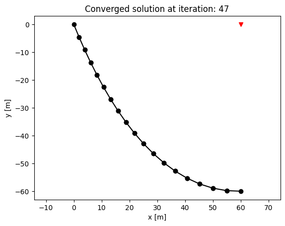
if CONV == 1:
    for iElem in np.arange(0, nElem):
            NodeLeft = int(Element[iElem, 0])
            NodeRight = int(Element[iElem, 1])
            DofsLeft = 2*NodeLeft 
            DofsRight = 2*NodeRight
            plt.plot([NodeCoord[NodeLeft][0] + u[DofsLeft], NodeCoord[NodeRight][0] + u[DofsRight]], 
                        [NodeCoord[NodeLeft][1] + u[DofsLeft + 1], NodeCoord[NodeRight][1] + u[DofsRight + 1]], '-ok')
            
    # plot the supports
    plt.plot(D, 0, 'vr')
    plt.axis('equal')
    plt.xlabel("x [m]")
    plt.ylabel("y [m]")
    plt.title("Converged solution at iteration: "+str(kIter))
else:
    print("Solution did not converge")

# Step 3: Solve the dynamic problem

Mass = m*lmax # Weight per element
C = 0.001*EA # just some damping

M = np.zeros((nDof*nDof))
M[0] = Mass                         # Add mass at the left node
M[nDof + 1] = Mass                  # Add mass at the left node
Pext[1] = Pext[1] - Mass*g          # Add weight to the left node
for iElem in np.arange(0, nElem):
        NodeLeft = int(Element[iElem, 0])
        NodeRight = int(Element[iElem, 1])
        DofsLeft = 2*NodeLeft 
        DofsRight = 2*NodeRight
        l0 = Element[iElem, 4]
        EA = Element[iElem, 3]
        M_elem = m*l0/6*np.array([[2, 0, 1, 0], 
                                    [0, 2, 0, 1], 
                                    [1, 0, 2, 0], 
                                    [0, 1, 0, 2]])
        # Assemble the matrices at the correct place
        # Get the degrees of freedom that correspond to each node
        Dofs_Left = 2*(NodeLeft) + np.arange(0, 2)
        Dofs_Right = 2*(NodeRight) + np.arange(0, 2)
        nodes = np.append(Dofs_Left , Dofs_Right)
        for i in np.arange(0, 4):
            for j in np.arange(0, 4):
                ij = nodes[i] + nodes[j]*nDof
                M[ij] = M[ij] + M_elem[i, j]
M = M.reshape((nDof, nDof))

def ub(t):
    return 5 * np.cos(2*t)
def dub_dt(t):
    return -10 * np.sin(2*t)
def dub_dt2(t):
    return -20 * np.cos(2*t)

from StringDynamicForces import StringDynamicForces
def ACCELERATIONS(t, U, NodeCoord, Element, FreeDof, FixedDof, C, M, Pext, TENSION_ONLY):
    nDof = len(U)
    u = U[:nDof//2]
    v = U[nDof//2:]

    # free & fixed array indices
    fx = FreeDof[:, np.newaxis]
    fy = FreeDof[np.newaxis, :]
    FixedDof = np.array(FixedDof)
    bx = FixedDof[:, np.newaxis]
    by = FixedDof[np.newaxis, :]

    # Calculate internal forces
    FintDyn = np.zeros((nDof))
    for iElem in np.arange(0, len(Element)):
        NodeLeft = int(Element[iElem, 0])
        NodeRight = int(Element[iElem, 1])
        DofsLeft = 2*NodeLeft 
        DofsRight = 2*NodeRight
        l0 = Element[iElem, 4]
        EA = Element[iElem, 3]
        NodePos = ([NodeCoord[NodeLeft][0] + u[DofsLeft], NodeCoord[NodeRight][0] + u[DofsRight]], 
            [NodeCoord[NodeLeft][1] + u[DofsLeft + 1], NodeCoord[NodeRight][1] + u[DofsRight + 1]])
        NodeVel = ([v[DofsLeft], v[DofsRight]], 
                    [v[DofsLeft + 1], v[DofsRight + 1]])
        if iElem == 0:
            # CHANGES HERE: Added ub and dub_dt
            NodePos = ([NodeCoord[NodeLeft][0] + u[DofsLeft] + ub(t), 
                        NodeCoord[NodeRight][0] + u[DofsRight]], 
                        [NodeCoord[NodeLeft][1] + u[DofsLeft + 1], 
                         NodeCoord[NodeRight][1] + u[DofsRight + 1]])
            NodeVel = ([v[DofsLeft] + dub_dt(t), v[DofsRight]], 
                        [v[DofsLeft + 1], v[DofsRight + 1]])
        Fint = StringDynamicForces(NodePos, NodeVel, EA, C, l0)
        FintDyn[DofsLeft:DofsLeft + 2] += Fint[0]
        FintDyn[DofsRight:DofsRight + 2] += Fint[1]

    # Calculate the new acceleration
    a = np.zeros((nDof//2))
    # CHANGES HERE: Added dub_dt2
    a[FreeDof] = np.linalg.solve(M[fx, fy], (Pext[FreeDof]-FintDyn[FreeDof]) 
                                            - np.dot(M[fx, by], [dub_dt2(t), 0, 0, 0])
                                )
    
    # Store the derivative of phase
    dU = np.append(v, a)
    #print("Time = "+str(t)+" s")
    return dU

v = u*0
U0 = np.append(u, v)
dt = 0.1
Tend = 10
tspan = np.arange(0, Tend, dt)

def odefun(t, U):
    # print(t) # Can add to follow progress - may take a few minutes
    return ACCELERATIONS(t, U, NodeCoord, Element, FreeDof, FixedDof, C, M, Pext, TENSION_ONLY)

sol = scp.solve_ivp(fun=odefun, t_span=[tspan[0], tspan[-1]], y0=U0, t_eval=tspan)  

%matplotlib inline
import time
from IPython import display

for iT in np.arange(0, len(sol.t)):
    try: 
        u = sol.y[:nDof, iT]
        for iElem in np.arange(0, nElem):
            NodeLeft = int(Element[iElem, 0])
            NodeRight = int(Element[iElem, 1])
            DofsLeft = 2*NodeLeft 
            DofsRight = 2*NodeRight
            plt.plot([NodeCoord[NodeLeft][0] + u[DofsLeft], NodeCoord[NodeRight][0] + u[DofsRight]], 
                        [NodeCoord[NodeLeft][1] + u[DofsLeft + 1], NodeCoord[NodeRight][1] + u[DofsRight + 1]], '-ok')
        # plot the supports
        plt.plot(D, 0, 'vr')     
        plt.axis('equal')
        plt.xlabel("x [m]")
        plt.ylabel("y [m]")
        #plt.savefig(f".././images/Module7/w7_t2ex_gif/shot{iT}.png")
        display.display(plt.gcf())
        display.clear_output(wait=True)
        plt.clf()
        time.sleep(0.01)
    except KeyboardInterrupt:
        break

u = sol.y[:nDof, -1]
for iElem in np.arange(0, nElem):
    NodeLeft = int(Element[iElem, 0])
    NodeRight = int(Element[iElem, 1])
    DofsLeft = 2*NodeLeft 
    DofsRight = 2*NodeRight
    plt.plot([NodeCoord[NodeLeft][0] + u[DofsLeft], NodeCoord[NodeRight][0] + u[DofsRight]], 
                [NodeCoord[NodeLeft][1] + u[DofsLeft + 1], NodeCoord[NodeRight][1] + u[DofsRight + 1]], '-ok')
# plot the supports
plt.plot(D, 0, 'vr') 
plt.axis('equal')
plt.xlabel("x [m]")
plt.ylabel("y [m]");

Now displaying the animated plots, gif conversion via https://ezgif.com/jpg-to-gif.