8.1. Key concepts#
Relationship between macro- and micro-scale#
The lack of pure homogeneity at a lower scale has a huge influence on the behaviour at the large scale. Small defects are known to often be the cause of catastrophic macroscopic failure, often linked to the failure of a brittle material due to crack propagation. Macro-scale properties often depend on micro-scale features encapsulated in what is named structure-property relationship. Even further, some macro-scale behaviour can emerge exclusively from the micro-scale such as strain localisation or mechanical size effect.
It is computationally impossible however to model those microscopic features when solving a macroscopic simulation as it requires a mesh resolution way too large to bridge the length scale separation (think about the TV resolution needed to resolve every strand of hair when displaying a person’s face! Even with 8K TV, we are not there yet…).
Separation of scales occurs when the macroscopic length scale is larger than the microscopic length scale by more than 3 orders of magnitude. Otherwise, concurrent/embedded multiscale method also exist but we will focus on the first kind, hierarchical (see differences highlighted in Fig. 8.1).
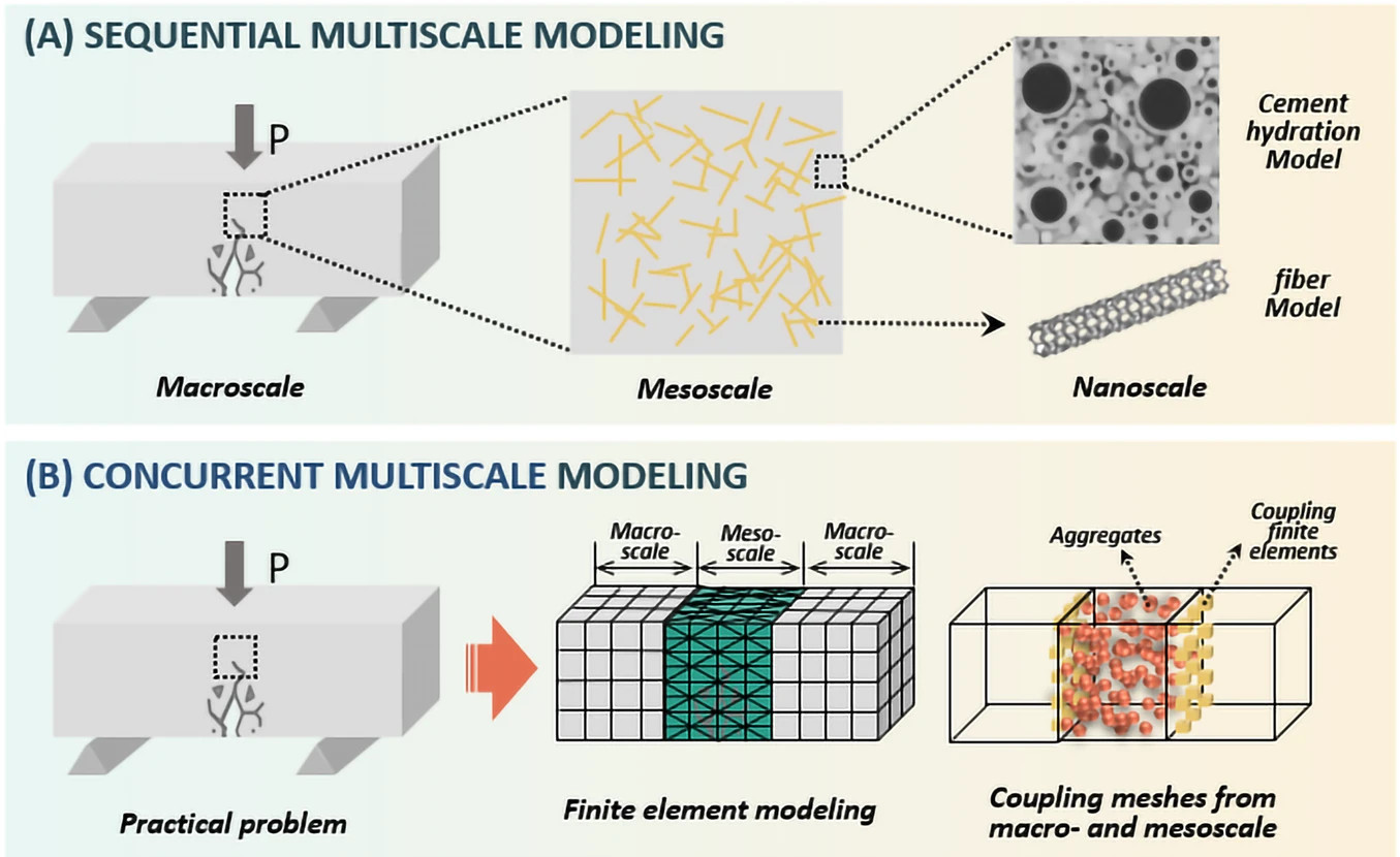
Fig. 8.1 Sequential vs concurrent multiscale modeling, applied to the fracturing problem of fiber-reinforced concrete. Figure from Wang et al. (2024)1.#
Because the scales are separated, the micromodel and macromodel need to be solved separately and coupled with a multiscale method. They are appropriately solved according to the scale considered. For example, while the microstructure is discretised at the micro-scale, the macro-scale is solved as a continuum (see Fig. 8.2).
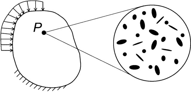
Fig. 8.2 Continuum macrostructure and heterogeneous microstructure associated with point P. Figure from Kouznetsova et al. (2001)2.#
To percolate information of the micro-scale to the macro-scale, we perform an upscaling using a homogenization method. The upscaled macroscopic response is called effective. Those multiscale methods are meant to couple the micro-scale and macro-scale models. In this first part we focus on the upscaling, which is a one-way coupling, upwards.
Categories of multiscale methods#
Different types of methods can be used to upscale. We can resort for example to simple empirical relationships which are the laws of mixtures. The first one from Voigt assumes that the effective medium is under a constant strain. For a two-phase medium, the effective value of the property is equivalent to setting two springs in parallel, and is expressed as:
Where \(\phi_1\) is the volume fraction of phase 1. For Reuss law, the assumption is constant force and similarly, the effective value of the property for a two-phase medium is equivalent to two springs in series and is expressed as
Those two formulas correspond respectively to kinematic or traction condition. Kinematic condition pushes the system to its maximal entropy and corresponds therefore to an upper bound of the effective property estimation, while the traction condition is oppositely the minimum. An applied interactive example is shown below.
When only interested in predicting failure, we can employ limit analysis which can consider more details of the microstructure. It can only derive however the upper and lower bounds of the solution. When trying to consider the exact microstructure, we need to resort instead to the computational methods. In this computational modelling book, we focus on that last option.
Representative Elementary Volume#
While the micro-scale is heterogeneous whether in structure or in property distribution, the application of multiscale methods can only be valid when the large scale is statistically homogeneous. We define as such a Representative Elementary Volume (REV) above which size the effective property of interest does not fluctuate. The REV is defined for the property to upscale and the length scale considered. When focusing on upscaling the microstructure, the length scale is the characteristic length of voids, inclusions, fibers or crystals depending on the material. For porous rocks for example, it is the average grain size. And studies show that the REV size for hydraulic conductivity of a rock is often larger than for its geometrical properties such as specific surface area or porosity (Mostaghimi et al., 20123).
A sample stops being statistically homogeneous when encountering a high length scale like fractures for example. Therefore, only unfractured samples can be homogenized (See \(V_{max}\) in Fig. 8.3). Still, we can upscale the effective response of a fracture network when we consider the fracture as the length scale of interest.
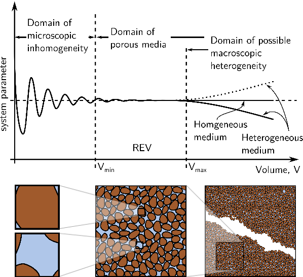
Fig. 8.3 Different scales of REV. Figure from Böttcher (2012) 4.#
When the structure is periodic such as for artificial materials like 3D-printed metamaterials, the REV is directly the unit cell and the upscaling is done using periodic boundary conditions. In the case of natural non-periodic REV, the REV size needs to be sufficiently large enough to eliminate boundary effects.
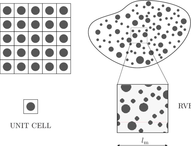
Fig. 8.4 Representative Elementary Volume for a periodic composite material (left) and for a random material (right). Figure from Nguyen et al. (2012)5.#
Averaging theorem#
Effective quantities are obtained by averaging the microscopic fields. The average of the quantity \(X\) over the domain \(\Omega\) is defined as:
For the relationship macro to micro, we obtain:
This relation is derived from the Hill-Mandel condition which expresses an irrefutable principle of thermodynamics. Hill’s lemma states that the energy has to be conserved across scales. As a consequence, the macroscopic work has to be equal to the average of the microscopic work. From this condition, the averaging of other quantities can be derived similarly.
At the microscopic scale, any quantity can be expressed as a fluctuating field around the averaged value:
Where \(\widetilde{X}\) is the fluctuation. Therefore we have:
This expression implies that the fluctuations need to average out on the domain for Eq. (8.1) to be valid. This is indeed the case when considering the domain size above REV, as per its definition. It showcases once more the need to consider a domain above the REV size for upscaling.
Upscaling#
To obtain an effective property, we refer to the macroscopic constitutive law. The law is inverted to compute the property using the macroscopic fields values obtained from our simulation. Not all fields need to be averaged because the value of the boundary condition imposed on the system to close it corresponds directly to the macroscopic value of this variable. The other macroscopic variables are obtained by homogenizing the microscopic fields heterogeneously distributed in the simulation result.
To give an example, we go through the steps of upscaling the Young’s modulus of a porous material:
Set up a numerical experiment of uniaxial mechanical test with displacement-control of a sample of the porous material above the REV size. The simulation solves for elasticity at the micro-scale. The macroscopic constitutive law for elasticity – Hooke’s law – reads as:
The macroscopic axial strain can be directly calculated from the prescribed displacement at the boundary.
The macroscopic axial stress is averaged from the microscopic axial stress over the full sample.
The effective Young’s modulus is calculated from Eq. (8.2).