PyJive workshop: material nonlinearity#
import matplotlib.pyplot as plt
import numpy as np

import os
import sys

pyjivepath = '../../../pyjive/'
sys.path.append(pyjivepath)

if not os.path.isfile(pyjivepath + 'utils/proputils.py'):
    print('\n\n**pyjive cannot be found, adapt "pyjivepath" above or move notebook to appropriate folder**\n\n')
    raise Exception('pyjive not found')

from utils import proputils as pu
import main
from names import GlobNames as gn

%matplotlib widget
# download additional files (if necessary)

import contextlib
from urllib.request import urlretrieve

def findfile(fname):
    url = "https://gitlab.tudelft.nl/cm/public/drive/-/raw/main/material/" + fname + "?inline=false"
    if not os.path.isfile(fname):
        print(f"Downloading {fname}...")
        urlretrieve(url, fname)

findfile("plasticity.pro")
findfile("voids.msh")
Plasticity model on a non-trivial 2D domain#
In this workshop, we look at the following geometry:
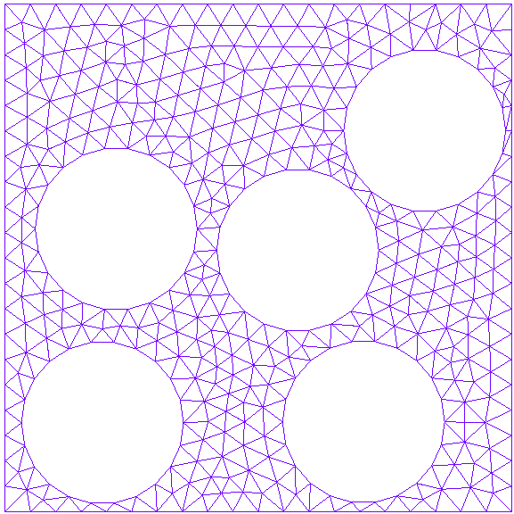
with Dirichlet boundary conditions that represent a state of global uniaxial tension, i.e. we pull this square-shaped domain on the right edge while keeping the left edge fixed horizontally and the bottom edge fixed vertically. The main model is a SolidModel and it is combined with a NonlinModule to perform nonlinear analysis, where the nonlinearity comes from the material model. A first version for this model in plasticity.pro. We run a displacement-controlled simulation for \(40\) time steps with props['model']['dispcontrol']['timeSignal'] = 't', which means the displacement at the right edge of the model is monotonically increasing. That will be adapted later on to explore more complex loading scenarios.
Task 1a: Run the model as is and look at the resulting force-displacement diagram.
The plasticity model has perfect plasticity (i.e. a constant yield stress), nevertheless, the load-displacement diagram displays a more gradual hardening behavior. Why does the finite element response not exactly mirror the material behavior for this case?
props = pu.parse_file('plasticity.pro')

globdat = main.jive(props)
The material model has a history variable \(\kappa\), which is a measure for accumulated plastic strain:
$$\kappa(t)=\displaystyle\int_0^t\sqrt{\frac{2}{3}\dot{\boldsymbol{\varepsilon}}^\mathrm{p}(t):\dot{\boldsymbol{\varepsilon}}^\mathrm{p}(t)}\,dt$$
Task 1b: Postprocessing
Analyze the results with the tools included in the cell below.
It is possible to show the evolution of displacements with the
ViewModule. This can module can be constructed in the notebook. How can you see from the evolution of the displacements that the material behavior is nonlinear?From
J2Material, we store inglobdatthe maximum value of the history variable \(\kappa\) throughout the whole domain \(\Omega\) after every time step. We can then plot this to see how \(\kappa\) is evolving in time. Do the results make sense?
# visualize displacements
view = globdat[gn.MODULEFACTORY].get_module('View','view')

props['view'] = {}
props['view']['plot'] = 'solution[dx]'
props['view']['deform'] = 1
props['view']['ncolors'] = 100
props['view']['interactive'] = 'True'
props['view']['colorMap'] = 'plasma_r'

view.init(props, globdat)
status = view.shutdown(globdat)

# plot history variable as function of time
plt.figure()
plt.xlabel('Time step')
plt.ylabel('$\max_\Omega(\kappa)$')
plt.plot(range(len(globdat['maxkappa'])),globdat['maxkappa'])
Unloading behavior#
Let us now run the same model, but change props['model']['dispcontrol']['timeSignal'] to include loading/unloading/reloading branches. More specifically, try to make the time signal reflect the following plot:
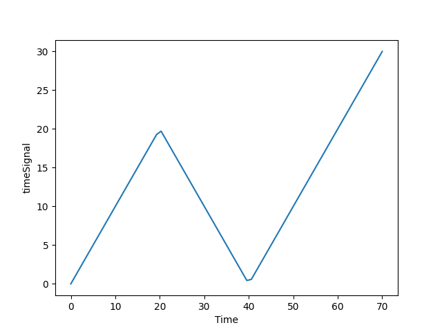
To do that, you can use the min() and max() functions. For instance, to create a single loading/unloading branch we could write
props['model']['dispcontrol']['timeSignal'] = 'min(t, 40-t)'
where t1 is the switching point. You can read this as being equivalent to:
if t < 40-t
    signal = t
else:
    signal = 40-t
Task 2: Loading/unloading behavior
Set up a case with unloading and reloading. For that you will need a nested expression with a combination of min and a max
Formulate a linear relation of for each three of the branches of the time signal visualized above
Define the time signal as a nested expression using
minandmaxRun the code, and check from the force displacement curve whether the boundary conditions work as intended
Perform further postprocessing of the displacement field and the maximum value of \(\kappa\)
Inspect the convergence data from the nonlinear solver. Most time steps need multiple iterations, but some time steps converge in one iteration. What is the reason for this?
props = pu.parse_file('plasticity.pro')

props['model']['dispcontrol']['timeSignal'] = '??'
props['nonlin']['nsteps'] = 70

globdat = main.jive(props)