Pyjive workshop: Applying constraints#
Preliminaries#
import matplotlib.pyplot as plt
import numpy as np
# download additional files (if necessary)

import contextlib
import os
from urllib.request import urlretrieve

def findfile(fname):
    url = "https://gitlab.tudelft.nl/cm/public/drive/-/raw/main/constraints/" + fname + "?inline=false"
    if not os.path.isfile(fname):
        print(f"Downloading {fname}...")
        urlretrieve(url, fname)

findfile("kmatrix.py")
Problem statement#
Consider the following 1-element problem composed of a single linear quadrilateral (Q4 or Quad4) element:
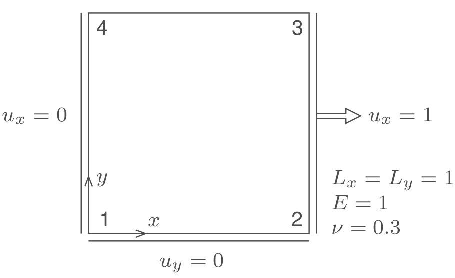
where you can also see several of the DOFs are constrained to either zero or non-zero values (Dirichlet constraints).
Using the correct shape functions \(\mathbf{N}\) and encapsulating our kinematic assumptions in \(\mathbf{B}\), we can use numerical integration to compute the stiffness matrix of this element. The resulting values are:
which is in this single element model also the global stiffness matrix.
Now recall we would like to use this matrix to solve for \(\mathbf{u}\):
which means \(\mathbf{K}\) should be invertible.
In the block below, try to directly invert \(\mathbf{K}\) using np.linalg.inv(). You can also try to multiply \(\mathbf{K}^{-1}\) by a force vector, say one containing some small Gaussian noise:
Task 1: Invert the matrix
Complete the code block below to invert \(\mathbf{K}\) and solve \(\mathbf{Ku}=\mathbf{f}\) with a random force vector with small numbers.
What do you observe for the values in \(\mathbf{K}^{-1}\) and \(\mathbf{u}\)?
from kmatrix import K

# try to invert K here

random_f = np.random.normal(scale=0.1,size=8)

# try to solve for u here
Introducing constraints#
There is clearly something missing in the model above. The huge matrix entries in \(\mathbf{K}^{-1}\) are a telltale sign of an (almost) singular matrix. This also makes physical sense: For now, this is a Q4 element floating in space. In order for a unique equilibrium to exist for any external force, we have to introduce supports.
To demonstrate how Dirichlet boundary conditions are applied in pyJive, we copy here parts of the Constrainer class that can be found in utils/constrainer.py:
class Constrainer:
    def __init__(self):
        self._dofs = []
        self._vals = []

    def add_constraint(self, dof, val):
        self._dofs.append(dof)
        self._vals.append(val)

    def constrain(self, k, f):
        kc = np.copy(k)
        fc = np.copy(f)

        for dof, val in zip(self._dofs, self._vals):
            for i in range(kc.shape[0]):
                if i == dof:
                    fc[i] = val
                else:
                    fc[i] -= kc[i, dof] * val

            kc[:, dof] = kc[dof, :] = 0.0
            kc[dof, dof] = 1.0

        return kc, fc
We now use the Constrainer to apply our BCs.
For assembling the element stiffness matrix \(\mathbf{K}\), we implicitly assumed the following DOF order:
That means our constraints look like:
Node |
Direction |
DOF index |
Value |
|---|---|---|---|
1 |
\(x\) |
0 |
0 |
1 |
\(y\) |
1 |
0 |
2 |
\(x\) |
2 |
1 |
2 |
\(y\) |
3 |
0 |
3 |
\(x\) |
4 |
1 |
4 |
\(x\) |
6 |
0 |
In the full code, we do not need to manually keep track of DOF indices. This bookkeeping is taken care of by the DofSpace class, and to retrieve a DOF index we only need to know the node index and the DOF direction.
For simplicity, we do it manually here.
Task 2: Constrain the problem
Use the code block below to tell the constrainer class what constraints are there for this problem
Run the following blocks to construct and inspect the constrained stiffness matrix and force vector
con = Constrainer()

# ...
# con.add_constraint(???,???)
# ...
The constrainer instance is now ready to give us the constrained matrix:
f = np.zeros(8)
Kc, fc = con.constrain(K, f)
We can take a look inside:
print('Constrained matrix\n',Kc)
print('Constrained force\n',fc)
Or have a qualitative look by plotting them:
fig = plt.figure(constrained_layout=True)

fig.suptitle('Stiffness matrix')
axs = fig.subplots(1, 2, sharey=True)
axs[0].imshow(K,vmin=-0.5,vmax=1)
axs[0].set_title('Unconstrained')
axs[0].set_xticks(range(0,8))
axs[1].imshow(Kc,vmin=-0.5,vmax=1)
axs[1].set_title('Constrained')
axs[1].set_xticks(range(0,8))
fig = plt.figure(constrained_layout=True)

fig.suptitle('Force vector')
axs = fig.subplots(1, 2, sharey=True)
axs[0].imshow(f.reshape((8,1)),vmin=-0.5,vmax=1)
axs[0].set_title('Unconstrained')
axs[0].set_xticks([])
axs[1].imshow(fc.reshape((8,1)),vmin=-0.5,vmax=1)
axs[1].set_title('Constrained')
axs[1].set_xticks([])
Note that here we use the size-preserving approach, with 1 entries on the diagonal of the constrained DOFs. We also keep the symmetry of \(\mathbf{K}\) by moving some terms to the right-hand side of the system.
Solving the system#
Task 3: Solve the constrained problem
Use the code block below to solve the constrained system of equations
Does the solution satisfy the constraints?
What are the values of the displacements that were unknown in this problem?
Are these displacement values in line with expectations?
Instead of storing it as a sparse matrix and solving the system (contrast it to how we do it in SolverModule), here we just invert it and multiply by \(\mathbf{f}\) for simplicity:
u = np.matmul(np.linalg.inv(Kc),fc)
print('Nodal displacements:',u)
Task 4: Compute support reactions
Partition matrix and vector in free (
f) and constrained (c) parts, using information from theConstraineron which DOFs are constrained.Code an expression that gives the reaction forces on constrained DOFs.
Do the results make sense for the given problem?
cdofs = con._dofs
fdofs = [i for i in range(len(K)) if i not in cdofs]

# kcf = K[np.ix_(???,???)]
# kcc = K[np.ix_(???,???)]

# uc  = u[???]
# uf  = u[???]

# reactions = ???
print('Support reactions:',reactions)
Task 5: Explore the `pyjive` source code
Check whether the functions in the
Constrainerare indeed the same as given below (seeutils/constrainer.py)From which place in the code is the
add_constraintfunction called?From which place in the code is the
constrainfunction called?