8.2. FE\(^2\)#
In some instances, standalone upscaling as described in the previous chapter is not possible. It is the case when the process to upscale is path- or history-dependent, such as irreversible processes like plasticity (see plastic localisations in Fig. 8.5). The micro-scale system requires therefore information from the macro-scale about the macroscopic state variables as the system evolves. Only then can the upscaled properties be fed to the macro-scale that can advance the simulation. The two scales are now coupled.
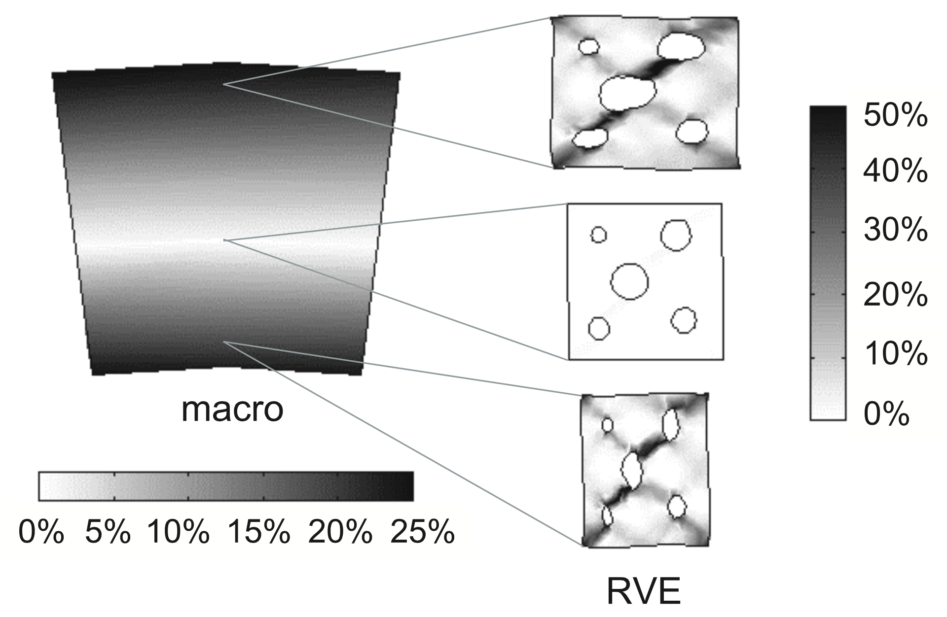
Fig. 8.5 Contour plots of the effective plastic strain in the deformed macrostructure and in three deformed RVEs, corresponding to different points of the macrostructure. Figure from Kouznetsova et al. (2001)1.#
The coupling can also be shortcutted for complex systems where the macroscopic constitutive law cannot be directly defined. Instead of upscaling the effective property, the upscaled macroscopic variables are directly transferred. This allows to not make any constitutive assumption about the material behaviour. When both scales are solved with finite element, these multiscale methods are called FE\(^2\), illustrated in Fig. 8.6.
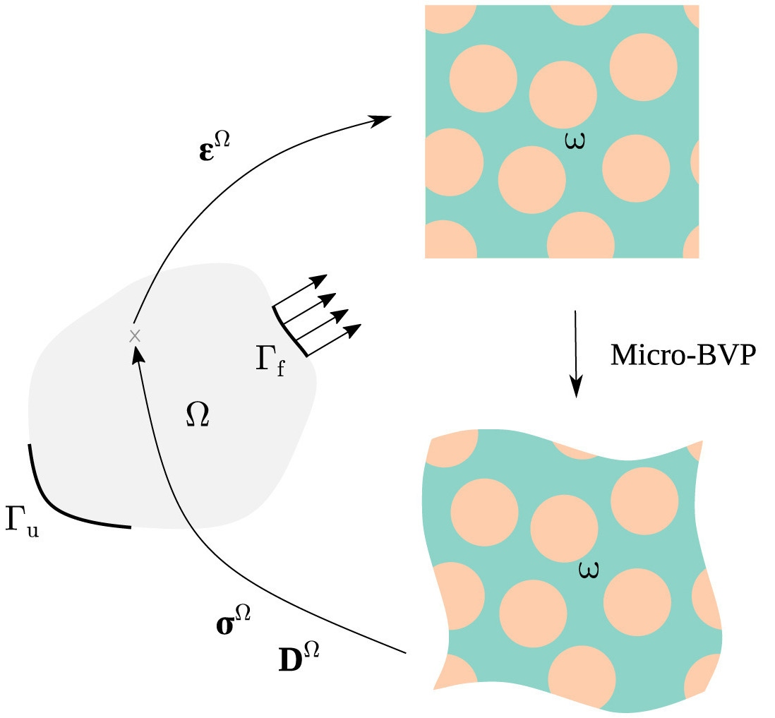
Fig. 8.6 Schematic of FE\(^2\) couplings. Figure from Maia et al. (2023)2.#
Information about the macroscopic state variables is downscaled under the form of a boundary condition. Voigt assumption of isostrain translates to imposing a constant deformation gradient on the boundary of the microstructure while Reuss assumption is to impose a constant stress. Periodic boundary conditions can also be adopted. Each setup satisfies Hill-Mandel condition given adequate microscopic field averaging (see Averaging theorem).
As the two simulations are hierarchical and therefore run sequentially, FE\(^2\) is not tightly coupled. Therefore, if the micromodel is nonlinear, we need to loop iteratively one timestep of the multiscaling, similarly to solving a nonlinear FEM problem (see Incremental-iterative algorithms), to reach convergence of the solution.
Typical set up for FE\(^2\) is to run that multiscale loop at every Gauss point of the mesh (see Fig. 8.7), so that the full field is determined through upscaling. Each multiscale loop can be run in parralel which allows to accelerate the multiscale simulation which is otherwise computationally very heavy.
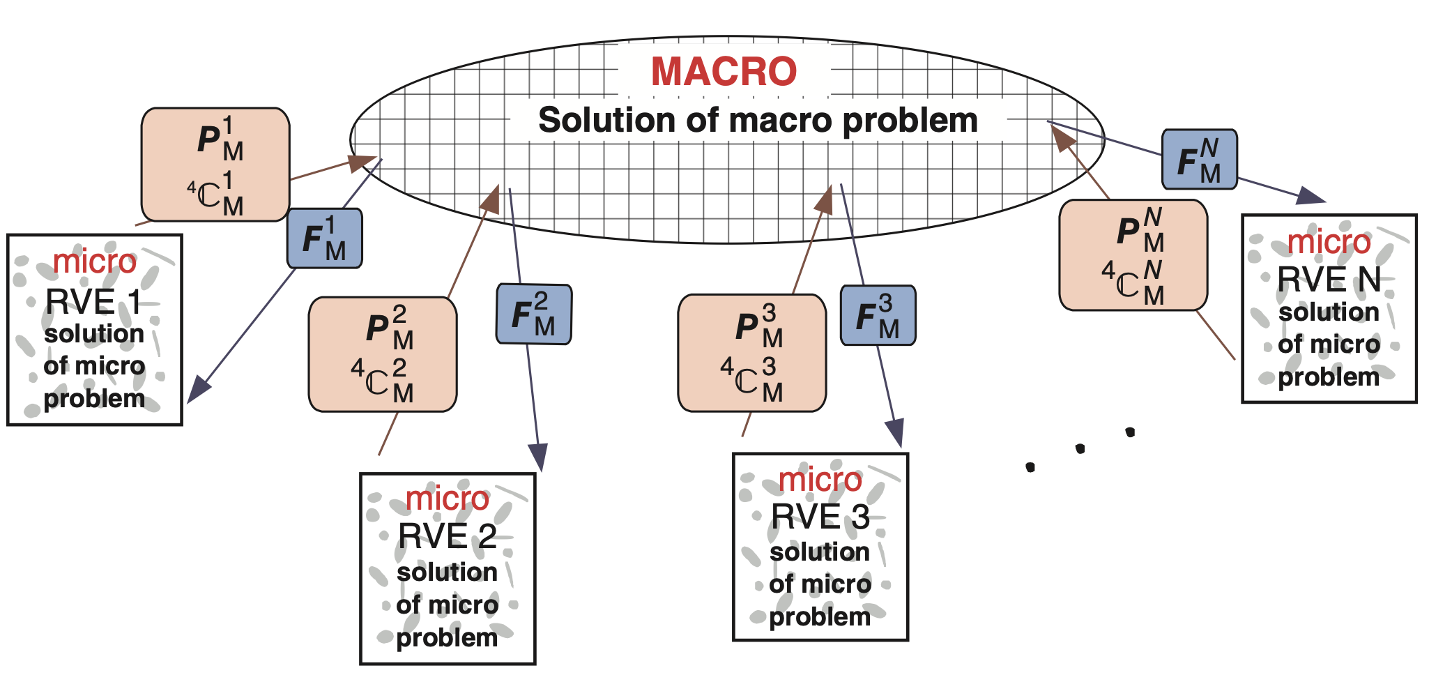
Fig. 8.7 Schematic of FE\(^2\) for every Gauss point. Figure from Geers et al. (2017)3.#
It is also possible to run a multiscale loop only in certain regions of the domain to enrich certain parts with micro-scale information. Commonly this is done on shear bands/fractures/faults, i.e. flat interfaces captured as lower dimensional elements and commonly implementing a cohesive zone model, as illustrated in Fig. 8.8. The microscale loop can return the displacement jump for example or oppositely receive the displacement jump and return the traction.
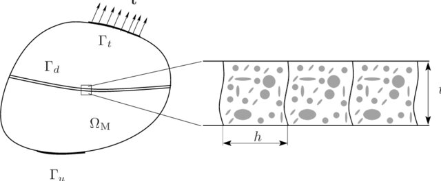
Fig. 8.8 Lower-dimensional fracture resolved with FE\(^2\). Figure from Nguyen et al. (2012)4.#