Pyjive workshop: Poisson and diffusion problems#
In this workshop, we simulate diffusion problems with pyJive. We will solve the steady state solution with the PoissonModel and then a transient problem with the DiffusionModel. Note that we use object-oriented programming here to relate the DiffusionModel to the PoissonModel implementation. DiffusionModel inherits functionality from PoissonModel and adds to it.
Preliminiaries#
%load_ext autoreload
%autoreload 2
%matplotlib widget

import contextlib
import os
from urllib.request import urlretrieve

import matplotlib.pyplot as plt
import numpy as np

import sys
pyjivepath = '../../../pyjive/'
sys.path.append(pyjivepath)

if not os.path.isfile(pyjivepath + 'utils/proputils.py'):
    print('\n\n**pyjive cannot be found, adapt "pyjivepath" above or move notebook to appropriate folder**\n\n')
    raise Exception('pyjive not found')

import main
from utils import proputils as pu
from names import GlobNames as gn
The autoreload extension is already loaded. To reload it, use:
  %reload_ext autoreload
# download input files (if necessary)

def findfile(fname):
    url = "https://gitlab.tudelft.nl/cm/public/drive/-/raw/main/diffusion/" + fname + "?inline=false"
    if not os.path.isfile(fname):
        print(f"Downloading {fname}...")
        urlretrieve(url, fname)

findfile("poisson.pro")
findfile("mesh.msh")
findfile("diffusion.pro")
1. Poisson problem#
First, solve a Poisson problem, which is the steady-state solution of a diffusion problem. A Poisson problem is specified in poisson.pro.
Task 1.1: Run code block and inspect results
Use the provided poisson.pro and mesh.msh files to solve a Poisson problem with pyJive. Inspect the input file and the solution. What are the boundary conditions at the four edges of the square domain? And what about interior boundary around the holes?
# parse input file and run analysis in a single line

globdat = main.jive(pu.parse_file('poisson.pro'))
2. Diffusion problem#
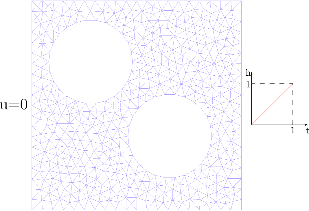
We will analyze the time-dependent problem visualized below, where boundary conditions change over time.
Task 2.1: Inspect the input file for the diffusion problem
Next, we will use the provided diffusion.pro and mesh.msh files to run the diffusion problem with pyJive. In the problem as provided, we run the problem for \(200\) time steps with \(\Delta t = 0.01\), with a total time of \(T=2\).
Compared to
poisson.pro, the input filediffusion.proa different model is specified underpdeand a different module undersolver. In both parts, additional inputs are specified. What is the meaning of these?Can you figure out from
diffusion.prowhat should to the boundary condition on the right for \(t>1\)?
Now we can run the code and inspect the results as visualized by the viewmodule. For that, you can use the slider to move back and forth in time.
globdat = main.jive(pu.parse_file('diffusion.pro'))
Task 2.2: Where is the $\mathbf{K}-matrix evaluated?
If you look at the file diffusionmodel.py, you see the \(\mathbf{M}\)-matrix is assembled there. However, the \(\mathbf{K}\)-matrix is not. Looking at trapezoidalmodule.py, you can see that both the \(\mathbf{M}\) and \(\mathbf{K}\) matrix are needed.
What are the respetive actions for assembly of \(\mathbf{K}\) and \(\mathbf{M}\)?
How often are the matrices assembled in the entire simulation?
How and where is the \(\mathbf{K}\)-matrix assembled?
Task 2.3: Investigate time step dependence
In the code block below some additional lines of code are provided for adapting the time step size. We will investigate the behavior of the finite element solver for increased time step size:
Modify the time step size from \(0.01\) to \(0.02\) and see what happens
Find the largest time step size for which the results are still good
Then set
props['solver']['theta'] = 1.0and repeat this exerciseWith \(\theta=1\) is is possible to run the simulation long enough to approach the steady state solution. Can you get a result that is close to the one obtained earlier with the Poisson equation?
Note: for compactness, from now on we wrap our main.jive() call in an environment that supresses the long printed output of the time stepper.
# define time increment and number of time steps
total_time = 2.0
delta_time = ??
nsteps = total_time / delta_time

# read input file
props = pu.parse_file('diffusion.pro')

# overwrite values related to the time increment
props['solver']['nsteps'] = nsteps
props['solver']['deltaTime'] = delta_time
props['model']['neum']['deltaTime'] = delta_time

# run code with output suppressed
with contextlib.redirect_stdout(open(os.devnull, "w")):
    globdat = main.jive(props)
Task 2.4: Perform a convergence study
In the code block below additional lines of code are provided for repeating the simulation with different time step sizes (and the same final \(t\)). With this we can investigate what time step size gives good accuracy. Suppose we are interested in the averaged temperature over the domain at \(t=2\), then we need to choose \(\Delta t\) sufficiently small to get accurate results. Even if the time-integration scheme is stable, accuracy can be an issue.
Complete the code block to perform a time-step convergence study.
Repeat this convergence study for different values of \(\theta\).
TIP: You can plot your results with matplotlib, with num_steps as x-axis.
ADVANCED TIP: Make a log-log plot of the error and compare the convergence behavior values of \(\theta\) in a single graph
def run_model(props):

    with contextlib.redirect_stdout(open(os.devnull, "w")):
        globdat = main.jive(props)

    return np.average(globdat[gn.STATE0])

total_time = 2

num_steps = [ 1,2,3,4,5,6,7,8,9,10,20,30,50,100 ]

vals = []

for step in num_steps:
    step_size = total_time / step

    props = pu.parse_file('diffusion.pro')

    # remove the 'view' part because it will generate too much output
    props.pop('view')

    # adapt inputs between different runs
    props['solver']['theta'] = 1.0
    props['solver']['nsteps'] = step
    props['solver']['deltaTime'] = step_size
    props['model']['neum']['deltaTime'] = step_size

    vals.append (run_model(props))