Pyjive workshop: NonlinModule#
In this workshop, we explore the functionality of the pyJive’s NonlinModule for nonlinear finite element simulations. We will explore the difference between force control and displacement control, look into the implementation of the incremental-iterative procedure in pyJive and see the influence of consistent linearization on convergence.
Preliminaries#
%load_ext autoreload
%autoreload 2

import matplotlib.pyplot as plt
import numpy as np

import os
import sys

pyjivepath = '../../../pyjive/'
sys.path.append(pyjivepath)

if not os.path.isfile(pyjivepath + 'utils/proputils.py'):
    print('\n\n**pyjive cannot be found, adapt "pyjivepath" above or move notebook to appropriate folder**\n\n')
    raise Exception('pyjive not found')

from utils import proputils as pu
import main
from names import GlobNames as gn
# download additional files (if necessary)

import contextlib
from urllib.request import urlretrieve

def findfile(fname):
    url = "https://gitlab.tudelft.nl/cm/public/drive/-/raw/main/nonlinmodule/" + fname + "?inline=false"
    if not os.path.isfile(fname):
        print(f"Downloading {fname}...")
        urlretrieve(url, fname)

findfile("square.pro")
findfile("square.msh")
\(J_2\) (Von Mises) plasticity for a 2D square-shaped domain#
We will work with the following single element model in 2D
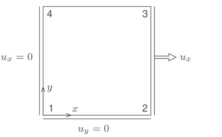
We use a plasticity model that introduces nonlinearity in the stress-strain relation.
For this two-dimensional model, we plot average displacements and forces at the right edge due to an applied load or displacement. Starting with a Neumann BC on the right, run the model below:
Task 1: Run the model as is and look at the resulting force-displacement diagram.
Can you identify the increments that were taken in the incremental-iterative procedure?
Does this correspond to what is defined in the input file?
Tip: In the input file, inputs are defined for more models than the number of models that is actually used in the simulation. We will make use of this additional input later. For now, look for the line with models = [ ... ] where it is specified which models are active.
props = pu.parse_file('square.pro')

globdat = main.jive(props)
Exponential hardening#
As you can see, the material had linear hardening for the model above. This is associated with the yield property in the input file, where \(\kappa\) is a measure for the amount of plastic strain. Now let us try exponential hardening.
Task 2: Run the model with exponential hardening.
Change the
yieldproperty to define an exponential hardening function: \(\sigma_\mathrm{y} = 120 - 80\exp\left(-\frac{\kappa}{0.015}\right)\).Run the model again and try to make sense of what happens.
Try to run the model for less steps and see at which point it crashes and why.
Try changing the time step size (
deltaTimeinneumann) to see if that helps.
props = pu.parse_file('square.pro')

globdat = main.jive(props)
Switching the loading scheme#
Task 3: Switch to displacement control
Try the same as above, but change props['model']['models'] to contain [solid, dispcontrol]. This will disable the original Neumann BC and switch to a displacement control strategy. Run the simulation again and see how far you can trace the equilibrium path now.
props = pu.parse_file('square.pro')

globdat = main.jive(props)
Unloading after plasticity#
Task 4: Change the time signal of the prescribed displacement
Try the same as above, but now modify the timeSignal property of dispcontrol to make the prescribed displacement unload after a number of steps. To achieve this you can set timeSignal = min(t,2*N-t), where you should substitute N by an integer representing the time step at which you would like to switch from loading to unloading. Make sure deltaTime=1.0 for this task.
Set the model to start unloading at time step
t=15. Can you explain what you see?Set the model to start unloading at time step
t=10. What is happening now?Finally, have the unloading start immediately after
t=1. What happened?
props = pu.parse_file('square.pro')

globdat = main.jive(props)
Modified Newton-Raphson in the NonlinModule#
Task 5: Adapt the NonlinModule to perform modified Newton-Raphson
Open
nonlinmodule.pyand adapt it such that in every iteration, the first computed stifness matrix from the time step is usedWhat happens to the convergence in displacement control?
Go back to exponential hardening in load control and set
['nonlin']['itermax'] = 50000and['neumann']['values'] = [3.0]. What happens to convergence?
Tips:
The
runfunction of of the NonlinModule is called once per time step. The iterative procedure to find a solution to the nonlinear system of equations can be found inside therunfunction.The action
GETMATRIX0is used to compute both \(K\) and \(\mathbf{f}_\mathrm{int}\). Don’t remove the action, because \(\mathbf{f}_\mathrm{int}\) still needs to be computed in every iteration. Find another way to ensure that the old matrix continues to be used.
props = pu.parse_file('square.pro')

globdat = main.jive(props)