Rod with elastic support#
In this chapter, the finite element derivation and implementation of rod extension (the 1D Poisson equation) is presented. A simple single purpose python implementation has also been given on the Finite element implementation page. In this exercise, you are asked to do the same for a slightly different problem.
A modification to the PDE: continuous elastic support#
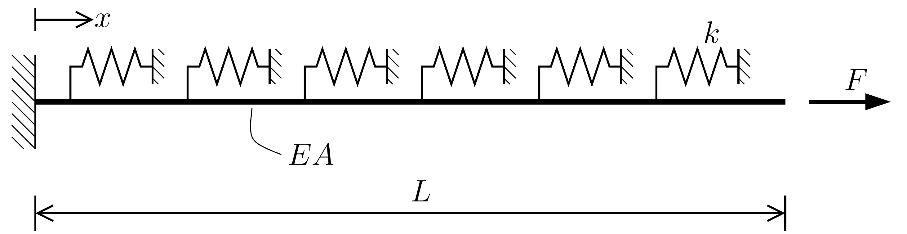
For this exercise we still consider a 1D rod. However, now the rod is elastically supported. An example of this would be a foundation pile in soil.
The problem of an elastically supported rod can be described with the following differential equation:
with:
This differential equation is the inhomogeneous Helmholtz equation, which also has applications in dynamics and electromagnetics. The additional term with respect to the case without elastic support is the second term on the left hand side: \(ku\).
The finite element discretized version of this PDE can be obtained following the same steps as shown for the unsupported rod in the book. Note that there are no derivatives in the \(ku\) which means that integration by parts does not need to be applied on this term. Using Neumann boundary condition (i.e. an applied load) at \(x=L\) and a constant distributed load \(f(x)=q\), the following expression is found for the discretized form:
Task 1: Derive the discrete form
Derive the discrete form of the PDE given above. You can follow the same steps as in the book for the term with \(EA\) and the right hand side, but now carrying along the additional term \(ku\) from the PDE. Show that this term leads to the \(\int\mathbf{N}^Tk\mathbf{N}\,dx\) term in the \(\mathbf{K}\)-matrix.
Modification to the FE implementation#
The only change with respect to the procedure as implemented in the book is the formulation of the \(\mathbf{K}\)-matrix, which now consists of two terms:
To calculate the integral exactly we must use two integration points.
Task 2: Code implementation
The only change needed with respect to the implementation of the book is in the calculation of the element stiffness matrix. Copy the code from the finite element implementation page and add the term related to the distributed support in the right position.
Use the following parameters: \(L=3\) m, \(EA=1000\) N, \(F=10\) N, \(q=0\) N/m (all values are the same as in the book, except for \(q\)). Additionally, use \(k=1000\) N/m\(^2\).
Remarks:
- The function
evaluate_Nis already present in the code in the book - The
get_element_matrixfunction already included a loop over two integration points - You need to define $k$ somewhere. To allow for varying $k$ as required below, it is convenient to make $k$ a second argument of the
simulatefunction and pass it on to lower level functions from there (cf. how $EA$ is passed on)
Check the influence of the distributed support on the solution:
- First use $q=0$ N/m and $k=1000$ N/mm$^2$
- Then set $k$ to zero and compare the results
- Does the influence of the supported spring on the solution make sense?
# YOUR_CODE_HERE
Task 3: Investigate the influence of discretization on the quality of the solution
- How many elements do you need to get a good solution?
- How about when the stiffness of the distributed support is increased to $k=10^6$ N/m$^2$
# YOUR_CODE_HERE
End of notebook.
© Copyright 2023 MUDE Teaching Team TU Delft. This work is licensed under a Creative Commons Attribution-NonCommercial-ShareAlike 4.0 International License.