Modelling precipitation

4.3. Modelling precipitation#

4.3.1. Spatial variation of rainfall#

Spatial variation of rainfall can be extremely important in hydrology because of spatially varying soil properties and land use types. The interplay between rainfall spatial variability and the stream channel network topology of a catchment can also have a large impact on its hydrologic behaviour. It is therefore important to characterize this spatial variability of rainfall to be able to draw conclusions on the behaviour of a catchment, in particular during extreme events. The variogram can be used to describe this spatial variability in a statistical manner. A variogram (which is short for semivariogram) is a geostatistical tool to describe the spatial variation of a field (rainfall in this case). It is often assumed that the spatial rainfall field is statistically stationary (the mean, variance, and spatial correlation of the field are independent of the location in space) and isotropic (the spatial correlation does not depend on direction). The correlation of the field at two points in space can then be expressed as a function of only the distance between these two points (i.e., independent of the position and direction).

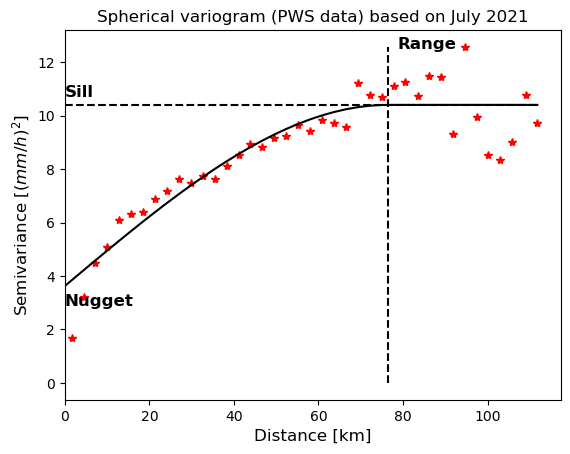
../_images/sphericalvariogram.png — Fig. 4.19 Example of a spherical variogram with parameters based on hourly rainfall observations from Personal Weather Stations (PWS) around the Geul, Rur and Vesdre catchments in July 2021. PWS data are extracted using the Netatmo API (https://dev.netatmo.com/apidocumentation) and filtered using part of the quality control algorithm (high influx and faulty zeroes) from De Vos et al. (2019). The circles represent the binned semi-variance. The solid line is the fitted spherical variogram using a least squares method. The horizontal dashed line is the sill, the vertical dashed line is the range, and the nugget is the y-intercept. (De Vos *et al.*, 2019)#

The semivariogram ($\gamma (d)$) is defined as half the variance of the difference between the field at two points ($p_{1}$ and $p_{2}$)

(4.5)#\[ \gamma (d)=\frac{1}{2}\mathrm{Var}\left[ R(p_{1})-R(p_{2})\right] \quad \text{[L$^{2}$/T$^{2}$]} \]

where $d=\left| p_{1}-p_{2}\right|$, and $R$ is the rainfall depth [L/T].

Empirical variograms are often used in spatial interpolation of rainfall fields. Each of the semivariances is assigned to a distance class. Then the mean semivariance is computed for each class. Subsequently, a variogram model is fitted to the mean semivariances. For instance, a spherical variogram is fitted to empirical variograms computed from a spatial rainfall field. This spherical variogram has some properties that can easily be interpreted. The spherical variogram has the following form

(4.6)#\[\begin{split} \gamma(d)= \begin{cases} C_0 + C [\frac{3}{2} \frac{d}{r} - \frac{1}{2} (\frac{d}{r})^3], & \text{if $d \le r$}.\\ C_0 + C, & \text{if $d>r$}. \end{cases} \end{split}\]

where $C_{0}$ is the nugget, $C_{0}+C$ is the sill and $r$ is the range (Fig. 4.19). The nugget is basically the variance at zero distance, which can be interpreted as very-fine scale variability or as measurement uncertainty. The sill is the variance at very large distances. The range is the distance at which the variance does not increase any more, which is equivalent to the distance beyond which the field is (nearly) completely decorrelated.

# Note that the code cells below is used for the website only.

Exercise 4.6

How does the range of a variogram of Dutch rainfall change during the year?

4.3.2. Spatial interpolation#

For most applications, it is not useful to know the rainfall intensities and sums at the meteorological stations alone; hydrologists usually want to know how much rain fell on an entire catchment. Several techniques can be used to interpolate between point measurements and obtain catchment total rainfall sums (also called catchment average rainfall, because rainfall is usually expressed in depths (mm) and not in volumes):

4.3.2.1. Arithmetic mean#

In this method, the rainfall of all stations in a catchment is averaged to obtain the catchment average precipitation:

(4.7)#\[ \overline{R} = \frac{1}{N} \sum^N_{j=1} R_j \quad \text{[L]} \]

with $\overline{R}$ the catchment average rainfall [mm], $N$ the number of stations [-] and $R_j$ the rainfall measured by each rain gauge [mm]. Of course, this method is very simple but not very accurate, because stations may not be uniformly distributed and the network density is often sparse.

4.3.2.2. Thiessen polygons#

Thiessen polygons area also called Voronoi diagrams in more general mathematical applications. This method is similar to the arithmetic mean method, but in the Thiessen polygon method not all stations receive the same weight:

(4.8)#\[ \overline{R} = \sum^N_{j=1} \omega_j \cdot R_j \quad \text{[L]} \]

where $\omega_j$ is the weight of each station [-]. To obtain the weights, the catchment area is divided into sub-areas, which are located around rain gauges (see Figure Fig. 4.20). From each point within the sub-area around a certain rain gauge, that particular rain gauge is closer than any other rain gauge. The weight of a rain gauge $\omega$ is the fraction of the total catchment area belonging to that rain gauge:

(4.9)#\[ \omega_j = \frac{A_j}{A_{total}}. \quad \text{[-]} \]

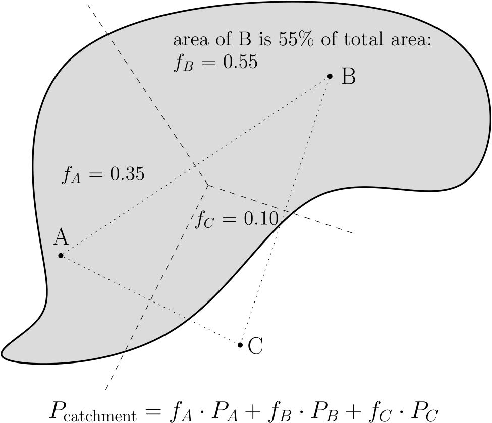
../_images/Thiessen-1.png — Fig. 4.20 Example of the construction of Thiessen polygons. First lines are drawn between the rain gauges $A$, $B$ and $C$ (dotted). Through the middle of these lines, perpendicular bisectors (*middelloodlijnen*) are drawn (dashed). These lines are the edges of the sub-areas belonging to each rain gauge.#

4.3.2.3. Elevation classes#

This method is applied in mountainous areas, where precipitation increases strongly with elevation. The precipitation at a certain location in the catchment in mountainous areas is more likely to be similar to that from a rain gauge at the same elevation than from a rain gauge nearby.

The available rain gauges are divided into elevation classes. With a digital elevation model or map the catchment area is divided into the same classes. The catchment average precipitation can be obtained from $N$ elevation classes by equation (4.8), with now $\omega_j$ the weight of each elevation class (the fraction of the total catchment area belonging to that class) [-] and $R_j$ the mean rainfall measured by all rain gauges in each elevation class [mm]. An example is given in Table 4.1.

When there is a large difference between windward side (NL: loefzijde) and leeward side (NL: lijzijde) one should also take the exposition to the wind

Table 4.1 Computing catchment average precipitation with elevation classes. Stations $B$, $C$ and $D$ are roughly at the same elevation, so they are combined into one class. The boundaries of the classes are halfway between the elevations of the stations.#
Station	Elevation [m]	Class	Boundaries [m]	Area [$\text{km}^2$]	Weight	Measured rainfall [mm]	Product [mm]
A	220	I	<310	11	0.55	10	5.5

4.3.2.4. Kriging#

The kriging method is more sophisticated than the previous methods because it takes into account the spatial dependence of rainfall. The catchment is divided into grids and on each grid point the rainfall is estimated from several rain gauges in the neighbourhood (Figure Fig. 4.21). The method requires a variogram model to determine the influence of each rain gauge at the grid point. A catchment average is simply obtained by averaging all grid points located within the catchment boundaries.

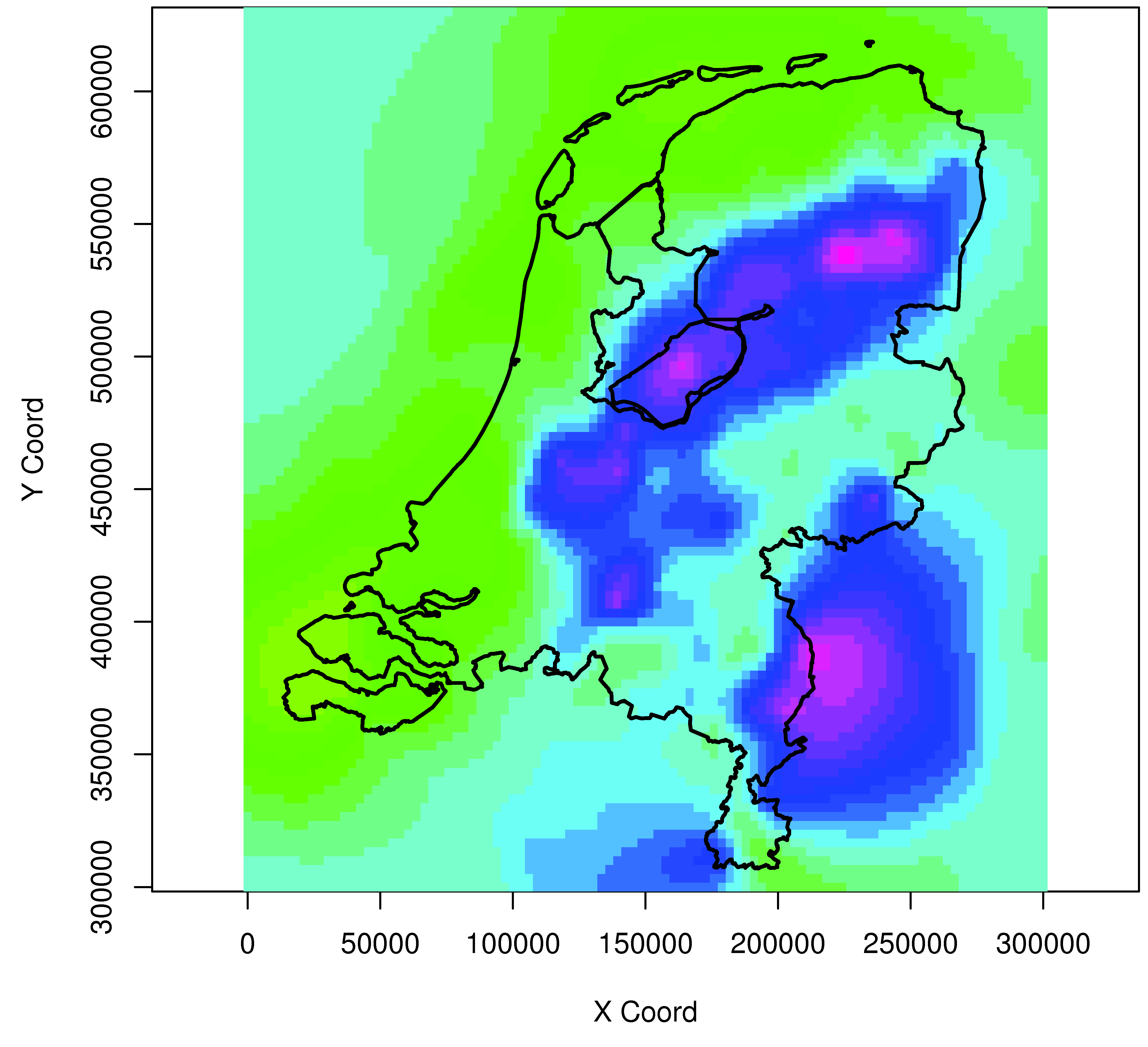
../_images/kriging.png — Fig. 4.21 Example of an interpolated rainfall field which has been constructed from daily rainfall depths from 324 manual rain gauges with the kriging method.#

4.3.3. Quality control#

The measured amount of precipitation differs between stations. This can be caused by the spatial variability described in the sections above or by measurement inaccuracies. Rain gauge measurement inaccuracies are often related to the exposition of the rain gauge. Sometimes rain gauges are located in rain shadows (under trees or close to walls) or too high. Rain gauges that are set up above the soil surface measure less precipitation than actually falls on the soil surface, because the air flows are disturbed by the presence of the rain gauge itself and some of the water droplets are blown over the rain gauge. To check rainfall data series for errors, several techniques can be used:

4.3.3.1. Rippl diagram#

In a Rippl diagram the cumulative precipitation sums of all stations are plotted against time. Rippl diagrams are not straight; wet periods increase the slopes of the curves and dry periods decrease the slope. If all stations would be the same, the curves would show the same reaction to wet and dry periods. In Fig. 4.22 an example of a Rippl diagram is shown.

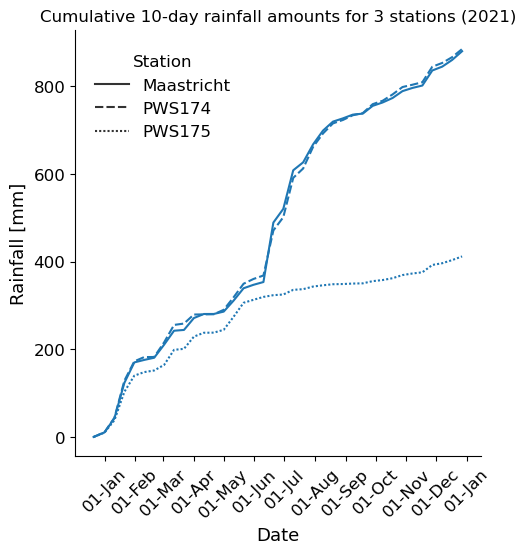
../_images/cumulative10-day.png — Fig. 4.22 Cumulative 10-day precipitation of three stations around the Geul catchment for 2021. Maastricht is the Automatic Weather Station (AWS) from the KNMI Data Platform (https://dataplatform.knmi.nl/dataset/access/neerslaggegevens-1-0). Personal Weather Stations (PWS) are extracted using the Netatmo API (https://dev.netatmo.com/apidocumentation) and filtered using part of the quality control algorithm (high influx and faulty zeroes). (De Vos *et al.*, 2019)#

4.3.3.2. Double-mass curves#

These are often used to check the consistency of rain gauge time series. In double-mass curves the cumulative time series of two rain gauges are plotted against each other (Fig. 4.23). When the curve is not on the 1:1-line, there is a systematic difference between the gauges. This may be due to instrumental artefacts, but also due to strong spatial rainfall gradients (especially if the gauges are far apart). A sudden change in the slope of the curve indicates that an abrupt change in one of the rain gauge time series has occurred.

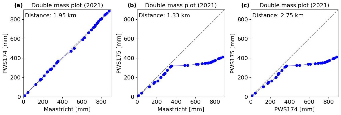
../_images/doublemasscurves.png — Fig. 4.23 Double mass curves for 10-day precipitation between three stations around the Geul catchment (same stations as in Fig. 4.22) for 2021. The curve reveals an abrupt change in the time series of PWS175 (b), which may be caused by an instrumental artefact.#

4.3.3.3. Ratios#

Spatial variability and differences in exposition cause differences in rainfall measurements. For example, station $A$ always catches 10% less than station $B$ because it is closer to the coast or on the leeward side of a mountain. The ratio between rainfall amounts caught at the two stations, in that case, will be quite stable in time. When plotting the ratio of two stations against time, one can see when there is a marked difference between the stations (Fig. 4.24). This difference may be a true difference (for example when convective rainfall events lead to large spatial variability), but may also be caused by measurement errors.

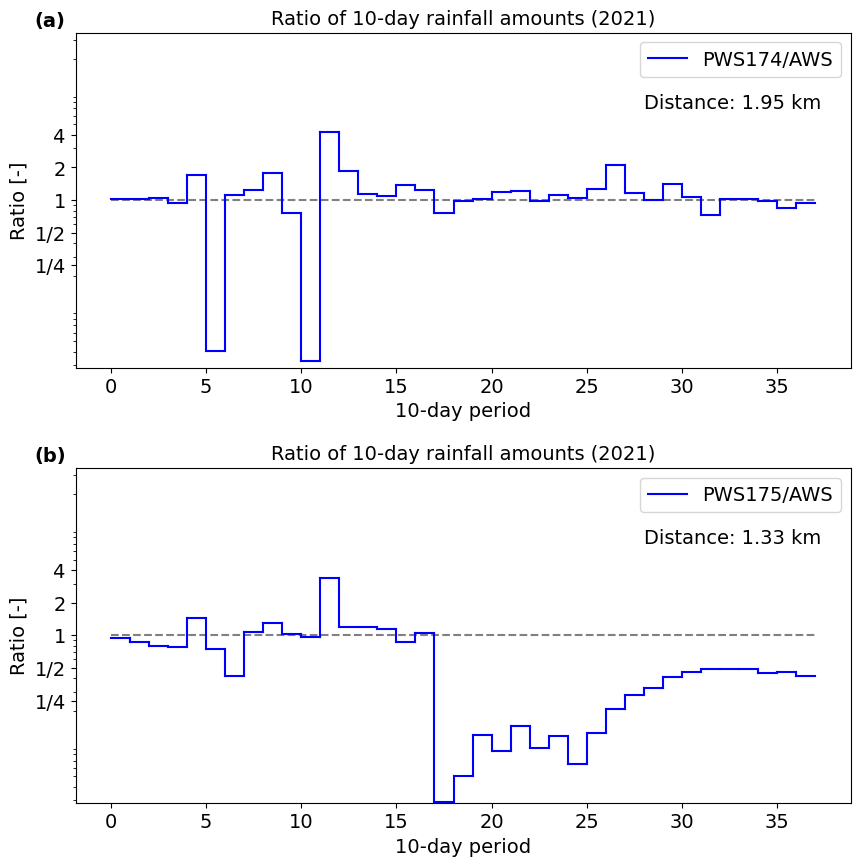
../_images/ratios.png — Fig. 4.24 Ratios of 10-day precipitation from three stations in the neighbourhood of the Geul catchment (same stations as in Fig. 4.22 & Fig. 4.23). The ratio reveals an abrupt shift in station performance of PWS175 (b).#

4.3.4. Gap-filling#

Precipitation time series are often not complete. Instruments can always fail or be out of operation for a while. These gaps can be filled by several methods.

4.3.4.1. Index-station method (rainfall-weigthed)#

According to this method, estimates are made with rainfall data from other stations in the vicinity (called index-stations), preferably in different directions around the station with missing data. Weights are attributed to the different stations, which depend on previously measured precipitation data. The weights are computed from mean values of the stations for corresponding periods. When 3 index-stations $A$, $B$ and $C$ are used, then the rainfall at the station with missing data $X$ is:

(4.10)#\[ R_x = \frac{1}{3} \left( \frac{\overline{R_X}}{\overline{R_A}} R_A + \frac{\overline{R_X}}{\overline{R_B}} R_B + \frac{\overline{R_X}}{\overline{R_C}} R_C \right) \quad \text{[L]} \]

in which $\overline{R_X}$, $\overline{R_A}$, $\overline{R_B}$, $\overline{R_C}$ are the mean values of the stations for a common period.

4.3.4.2. Index-station method (distance-weighted)#

Instead of the ratio of the means, the reciprocals of the distance (which is why this method is sometimes called ‘inverse distance’) can be used as weights. When the distances from $X$ to $A$, $B$ and $C$ are given by $r_A$, $r_B$ and $r_C$, respectively, then we find:

(4.11)#\[ R_X = \frac{\frac{R_A}{r_A}+\frac{R_B}{r_B}+\frac{R_C}{r_C}} {\frac{1}{r_A}+\frac{1}{r_B}+\frac{1}{r_C}}. \quad \text{[L]} \]

4.3.4.3. Linear regression#

Another way to fill gaps is to establish a relation between two stations. This relation is found by plotting the rainfall measurements of two stations against each other and fitting a line through the data. The relation of this line can then be used to estimate missing values with measurements of the other station. For example, in case of a linear relation, the rainfall at station $X$ can be estimated from the rainfall at station $A$ with:

(4.12)#\[ R_X = a + b \cdot R_A. \quad \text{[L]} \]

4.3.4.4. Isohyet method#

This method requires more work and is applied when differences between neighbouring stations are large. Rainfall is estimated from isohyetal maps (maps with lines with equal rainfall depths; isohyets). Strictly speaking it is not necessary to compute the isohyets first. We can also use an interpolation technique to estimate the missing values (such as Thiessen polygons).