7.4. Additional exercises#
For Exercise 7.7, you have two options: work with Python or with Excel. When applicable, python code is provided below each sub-question on this page. If you prefer working with Excel, please use the Python code below to generate an Excel file with the required data and answer the sub-questions in the chronological order. To generate the Excel file, simply copy the Python code and paste it into a notebook on your laptop. Remove the ‘#’ before the last code line to activate the generation of the Excel file. Once this is done, open the generated Excel file (located in the same folder as your notebook) in Excel.
Show code cell content
import numpy as np
import pandas as pd

years = np.array([1982, 1983, 1984, 1985, 1986])
QmaxY = np.array([211, 64, 99, 122, 165])
data = pd.DataFrame(index = years)
data['Qmax [m3/s]'] = QmaxY
nan_array = np.array([np.nan]*len(data['Qmax [m3/s]']))
data['Rank'] = nan_array
data['Probability of Exceedance'] = nan_array
data['Probability of non-Exceedance'] = nan_array
data['Reduced variate'] = nan_array
data['Return period [years]'] = nan_array
display(data)
#data.to_csv('Data.csv', index=False)
| Qmax [m3/s] | Rank | Probability of Exceedance | Probability of non-Exceedance | Reduced variate | Return period [years] | |
|---|---|---|---|---|---|---|
| 1982 | 211 | NaN | NaN | NaN | NaN | NaN |
| 1983 | 64 | NaN | NaN | NaN | NaN | NaN |
| 1984 | 99 | NaN | NaN | NaN | NaN | NaN |
| 1985 | 122 | NaN | NaN | NaN | NaN | NaN |
| 1986 | 165 | NaN | NaN | NaN | NaN | NaN |
Exercise 7.7
Extreme value analysis
You are asked to apply the Gumbel theory for extreme values to determine the design flow of a hypothetical river. No recent data is available, but you have found a very short time-series spanning over a few years in the 1980s, from which you have calculated the yearly maxima.
| Qmax [m3/s] | |
|---|---|
| 1982 | 211 |
| 1983 | 64 |
| 1984 | 99 |
| 1985 | 122 |
| 1986 | 165 |
a) First of all, fill in the table below.
Show code cell source
import numpy as np
import pandas as pd

years = np.array([1982, 1983, 1984, 1985, 1986])
QmaxY = np.array([211, 64, 99, 122, 165])
data = pd.DataFrame(index = years)
data['Qmax [m3/s]'] = QmaxY
nan_array = np.array([np.nan]*len(data['Qmax [m3/s]']))
data['Rank'] = nan_array
data['Probability of Exceedance'] = nan_array
data['Probability of non-Exceedance'] = nan_array
data['Reduced variate'] = nan_array
data['Return period [years]'] = nan_array
display(data)
| Qmax [m3/s] | Rank | Probability of Exceedance | Probability of non-Exceedance | Reduced variate | Return period [years] | |
|---|---|---|---|---|---|---|
| 1982 | 211 | NaN | NaN | NaN | NaN | NaN |
| 1983 | 64 | NaN | NaN | NaN | NaN | NaN |
| 1984 | 99 | NaN | NaN | NaN | NaN | NaN |
| 1985 | 122 | NaN | NaN | NaN | NaN | NaN |
| 1986 | 165 | NaN | NaN | NaN | NaN | NaN |
Answer Exercise 7.7 a
The table with solutions can be found in the code cell below.
Show code cell content
years = np.array([1982, 1983, 1984, 1985, 1986])
QmaxY = np.array([211, 64, 99, 122, 165])
data = pd.DataFrame(index = years)
data['Qmax [m3/s]'] = QmaxY
nan_array = np.array([np.nan]*len(data['Qmax [m3/s]']))
data['Rank [-]'] = data['Qmax [m3/s]'].rank(ascending=False)
data = data.sort_values('Rank [-]')
data['Probability of Exceedance [1/year]'] = data['Rank [-]']/(len(data['Rank [-]'])+1)
data['Probability of non-Exceedance [1/year]'] = 1 - data['Probability of Exceedance [1/year]']
data['Reduced variate [-]'] = -np.log(-np.log(data['Probability of non-Exceedance [1/year]']))
data['Return period [years]'] = (len(data.index.values) + 1) / data['Rank [-]']
data = data.round(3)
display(data)
| Qmax [m3/s] | Rank [-] | Probability of Exceedance [1/year] | Probability of non-Exceedance [1/year] | Reduced variate [-] | Return period [years] | |
|---|---|---|---|---|---|---|
| 1982 | 211 | 1.0 | 0.167 | 0.833 | 1.702 | 6.0 |
| 1986 | 165 | 2.0 | 0.333 | 0.667 | 0.903 | 3.0 |
| 1985 | 122 | 3.0 | 0.500 | 0.500 | 0.367 | 2.0 |
| 1984 | 99 | 4.0 | 0.667 | 0.333 | -0.094 | 1.5 |
| 1983 | 64 | 5.0 | 0.833 | 0.167 | -0.583 | 1.2 |
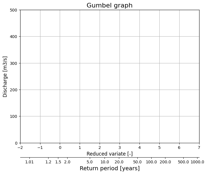
b) Next, make the Gumbel graph used to estimate the river flow for very large return periods. The code cell below provides you with a template for plotting the Gumbel graph.
Show code cell content
import matplotlib.pyplot as plt

# Plot
fig, ax1 = plt.subplots(figsize=(8,6))
ax1.set_title('Gumbel graph', fontsize='16')
ax1.set_xlim(-2, 7)
ax1.set_ylim(0,500)
ax1.set_ylabel('Discharge [m3/s]', fontsize='12')
ax1.set_xlabel('Reduced variate [-]', fontsize='12')
plt.grid()

# Set scond x-axis
ax2 = ax1.twiny()

# Decide the ticklabel position in the new x-axis,
# then convert them to the position in the old x-axis
newlabel = [1.01, 1.2, 1.5, 2., 5., 10., 20., 50., 100., 200., 500., 1000., 2000.] # labels of the xticklabels: the position in the new x-axis
k2_convert = lambda z: -np.log(-np.log(1-1/z))
newpos   = [k2_convert(z) for z in newlabel]   # position of the xticklabels in the old x-axis
ax2.set_xticks(newpos)
ax2.set_xticklabels(newlabel)

ax2.xaxis.set_ticks_position('bottom') # set the position of the second x-axis to bottom
ax2.xaxis.set_label_position('bottom') # set the position of the second x-axis to bottom
ax2.spines['bottom'].set_position(('outward', 36))
ax2.set_xlabel('Return period [years]',fontsize='14')
ax2.set_xlim(ax1.get_xlim());

Answer Exercise 7.7 b
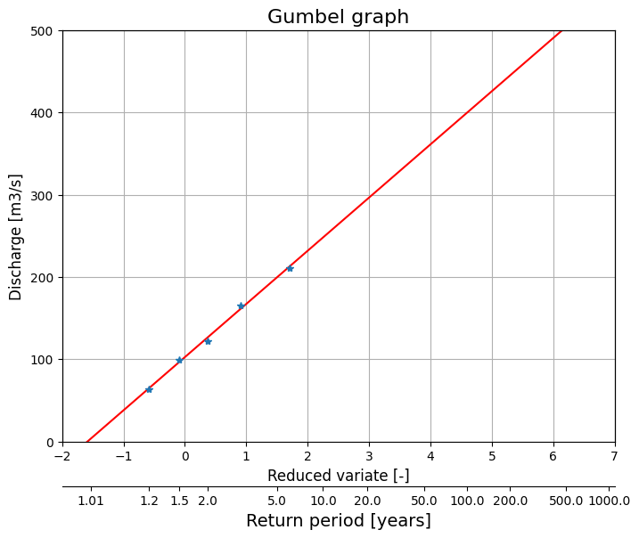
The Gumbel graph is generated in the code cell below. Don’t get intimated by the length of the code, a big the part of the code below is only used to create the axis labels and make the graph look nicer!
Show code cell content
import matplotlib.pyplot as plt

years = np.array([1982, 1983, 1984, 1985, 1986])
QmaxY = np.array([211, 64, 99, 122, 165])
data = pd.DataFrame(index = years)
data['Qmax [m3/s]'] = QmaxY
nan_array = np.array([np.nan]*len(data['Qmax [m3/s]']))
data['Rank [-]'] = data['Qmax [m3/s]'].rank(ascending=False)
data = data.sort_values('Rank [-]')
data['Probability of Exceedance [1/year]'] = data['Rank [-]']/(len(data['Rank [-]'])+1)
data = data.round(3)
data['Probability of non-Exceedance [1/year]'] = 1 - data['Probability of Exceedance [1/year]']
data['Reduced variate [-]'] = -np.log(-np.log(data['Probability of non-Exceedance [1/year]']))
data['Return period [years]'] = (len(data.index.values) + 1) / data['Rank [-]']

X = data['Reduced variate [-]']
y = data['Qmax [m3/s]']

# Computing the coefficients of the regression line (y = mx + b)
X_mean = np.mean(X)
y_mean = np.mean(y)

# Calculating the slope (m)
numerator = np.sum((X - X_mean) * (y - y_mean))
denominator = np.sum((X - X_mean) ** 2)
slope = numerator / denominator

# Calculating the intercept (b)
intercept = y_mean - slope * X_mean

# Plot
X_plot = np.linspace(-2, 7, 100)
fig, ax1 = plt.subplots(figsize=(8,6))
ax1.set_title('Gumbel graph', fontsize='16')
ax1.plot(X_plot, slope * X_plot + intercept, color='red', label='Regression Line')
ax1.plot(data['Reduced variate [-]'], data['Qmax [m3/s]'], '*')
ax1.set_xlim(-2, 7)
ax1.set_ylim(0,500)
ax1.set_ylabel('Discharge [m3/s]', fontsize='12')
ax1.set_xlabel('Reduced variate [-]', fontsize='12')
plt.grid()

# Set scond x-axis
ax2 = ax1.twiny()

# Decide the ticklabel position in the new x-axis,
# then convert them to the position in the old x-axis
newlabel = [1.01, 1.2, 1.5, 2., 5., 10., 20., 50., 100., 200., 500., 1000., 2000.] # labels of the xticklabels: the position in the new x-axis
k2_convert = lambda z: -np.log(-np.log(1-1/z))
newpos   = [k2_convert(z) for z in newlabel]   # position of the xticklabels in the old x-axis
ax2.set_xticks(newpos)
ax2.set_xticklabels(newlabel)

ax2.xaxis.set_ticks_position('bottom') # set the position of the second x-axis to bottom
ax2.xaxis.set_label_position('bottom') # set the position of the second x-axis to bottom
ax2.spines['bottom'].set_position(('outward', 36))
ax2.set_xlabel('Return period [years]',fontsize='14')
ax2.set_xlim(ax1.get_xlim());

c) Consider only one year. According to the table (i.e. without applying a Gumbel fit), what is the probability that the annual maximum river flow exceeds the maximum flow measured in 1985?
Answer Exercise 7.7 c
From the table above, the probability can be found to be equal to 0.500.
d) Consider only one year. According to the table (i.e. without applying a Gumbel fit), what is the probability that the annual maximum river flow is lower than the maximum flow measured in 1984?
Answer Exercise 7.7 d
From the table above, the answer is 0.333.
e) Based on the Gumbel distribution, estimate the river flow corresponding to a return period of 55.1 years.
Answer Exercise 7.7 e
In the table above, the discharge corresponding to a return period of 55.1 years is equal to 361.2 \(\frac{\text{m}^3}{\text{s}}\).
Exercise 7.8
True or false?
# Note that the code cells below is used for the website only.
