2.4. Application: Reservoirs

2.4.1. Introduction

Storage of water can take place both on the surface and underground. However, when we think of a reservoir, we usually envision above-ground storage, such as in a closed valley where a reservoir is created after closure, forming a dammed lake. Nevertheless, flat areas like The Netherlands also have reservoirs. For instance, the Biesbosch basins serve as storage for river water used as drinking water, and the IJsselmeer, Delta basins, and polder waters also have a reservoir function. Dikes play the role of water barriers in these reservoirs, similar to the valley walls in a dammed lake.

The principle of a reservoir is as follows: during periods when the available water exceeds the quantity required for various purposes such as drinking water, irrigation, hydropower etc., the excess water can be stored until a period of water scarcity arrives. Additionally, a function of a reservoir can be the storage of high flows, which helps reducing the risk of downstream flooding. Sometimes, reservoirs are specifically constructed for this purpose.

In urban areas where water demand can fluctuate significantly throughout the day, many cities have distribution reservoirs (NL: distributiereservoirs) in their water supply systems. This allows them to adapt to daily fluctuations, enabling pump stations and purification facilities to operate at a relatively constant level. Thus, the primary function of a reservoir can be described as stabilizing the inflow or outflow of water, either by regulating variable natural flow or meeting the varying demands of end users.

2.4.2. Properties of a reservoir

Fig. 2.6 shows several general characteristics of a reservoir with a dam. The storage capacity can be determined based on its primary function and the associated conditions.

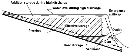
Fig. 2.6 Characteristics of a reservoir with a dam.

For a naturally formed reservoir, such as a valley closure, the capacity depends on the topography. The water surface varies with the water level, resulting in a non-linear relationship between the volume and the water level. By measuring the water surface at different water levels, an area-elevation curve (NL: oppervlakte-waterstandskromme) can be plotted. Integrating this curve gives the capacity curve (NL: capaciteitskromme) of the reservoir, which shows the variation of the storage volume as a function of the water level (see Fig. 2.7).

Fig. 2.7 Relationship between water surface and storage.

In Fig. 2.7:

(2.13)\[ S_1 = \int_{0}^{h_\text{1}} A(h)dh \quad \text{[L$^{3}$]} \]

where \(S_1\) represents the storage of the reservoir at water level \(h_1\), and \(A(h)\) is the surface area as a function of the water level.

It is evident that the entire volume of the reservoir cannot be used; the water below the lowest discharge opening is called the dead storage (NL: dode berging). This dead storage is not lost but ensures that the reservoir never runs dry, which could lead to significant environmental problems such as fish mortality, odor, and permanent ecological damage. Sedimentation can also occur in this part of the reservoir without reducing the useful storage volume. The maximum storage under normal conditions is typically determined by the height of the emergency spillway. During extreme flow conditions, the water level can still rise over the spillway, creating temporary additional storage, which can be substantial due to the maximum surface area (\(A_\text{max}\)). However, this additional storage cannot be retained and is uncontrollable.

In the original river channel, a variable amount of water was already stored, representing the amount of water present in that section of the river at a specific time. This storage is indicated in Fig. 2.6 by the line parallel to the riverbed. For purposes such as reducing the risk of downstream flooding, this original storage should not be considered when determining the increase in storage capacity. The increase in storage is referred to as the effective storage (NL: effectieve berging).

2.4.3. Water yield

An important characteristic of a reservoir, with water supply as its primary factor, is the relationship between storage capacity and yield (NL: leveringscapaciteit). The delivery capacity indicates how much water the reservoir can release during a specific period. This time frame can vary from a day for a small distribution reservoir to a year or longer for a large storage reservoir. The delivery capacity depends on the inflow into the reservoir and can therefore vary. The maximum amount of water that can be guaranteed during a critical dry period is referred to as the safe yield (NL: vaste leveringscapaciteit). Naturally, there is always a chance of an even drier period with a delivery capacity smaller than the safe yield. Since the safe yield cannot be precisely determined, probabilistic approaches are often used to make a good estimate. The maximum water delivery during a specific time interval is equal to the average inflow minus evaporation and leakage losses. If the inflow would always be equal to the water delivery (including evaporation and leakage losses), a reservoir would be unnecessary. However, with increased fluctuations in inflow or outflow, the required reservoir capacity also increases.

As a result, for each area and each reservoir, a different delivery capacity is targeted. Depending on the acceptable probability that the delivery capacity might not always be met, the capacity for the reservoir can be determined. A reservoir for urban water supply should only have a very small probability of not meeting the demand. However, an irrigation system may operate with a water delivery below the design capacity up to 20% of the time.

2.4.4. Capacity determination

The required capacity of a reservoir is determined by simulating the functioning of the reservoir over a certain period. In this process, the water balance equation is always used, in its simplest form:

(2.14)\[ {\text{d}\S \over \text{d}t} = I - O \quad \text{[L$^{3}$/T]} \]

For capacity determination, the summation of inflow (I) (NL: instroming) and outflow (O) (NL: uitstroming) is crucial. From the water balance equation, it is evident that the difference between these summations gives the storage:

(2.15)\[ \int_{t_0}^{t_1} I \text{d}t - \int_{t_0}^{t_1} O \text{d}t + S_0=S_\text{1} \quad \text{[L$^{3}$]} \]

As we will see later, the choices of the starting moment \(t_0\) and the assumption of storage \(S_0\) at \(t_0\) are critical for interpreting the method of capacity determination.

2.4.4.1. Graphical methods

There are various methods to determine the (required) capacity of a reservoir. Below, the two main graphical methods are described:

1. In Fig. 2.8, the cumulative sum of inflow minus withdrawals (including evaporation and leakage losses) is calculated as a function of time. The initial volume \(S_0\) is arbitrarily chosen at first. The difference between a valley and a peak can be used to deduce the required storage capacity. The difference between the highest peak and the lowest valley then gives the maximum required storage capacity. After this analysis, the lowest valley is positioned with a useful storage of \(0\).

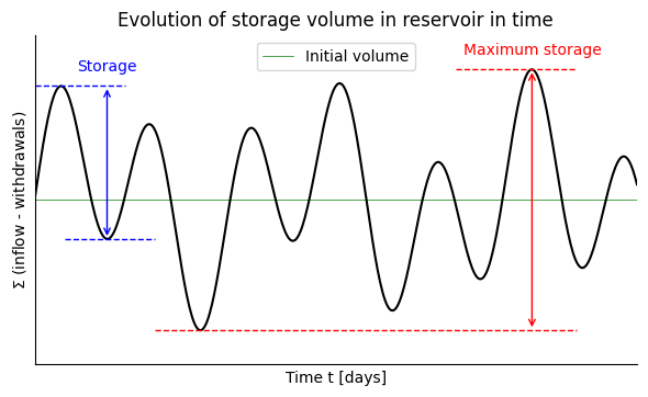
Fig. 2.8 Determination of the maximum required storage capacity.

2. For the determination of the capacity of a reservoir through which a river flows, the summation curve of inflow is often used, referred to as the Rippl diagram (Rippl, 1883) in this context. Summation of inflow results in a continuously non-decreasing line, with the slope at each point proportional to the inflow at that moment. Assuming that the water demand is constant and thus requires a constant supply, this can be represented by straight lines. These (tangent) lines (NL: raaklijnen) are shifted to touch the extreme points of the summation curve, as shown in Fig. 2.9 (\(A\), \(B\), and \(C\); at these points, filling the reservoir transitions to withdrawal). We assume that the reservoir is full at the starting moment (\(S_0 = S_\text{max}\)). From the point of contact, the water demand exceeds the inflow, and the storage decreases. Assuming that the reservoir is exactly full again when a demand line intersects the summation curve, the maximum distance between a demand line and the summation curve indicates the required capacity to meet the demand. In Fig. 2.9, this volume is represented by the distance \(FG\). The vertical distance between two consecutive demand lines (\(BH\)) represents the amount of water that can no longer be stored and is discharged via the emergency spillway.

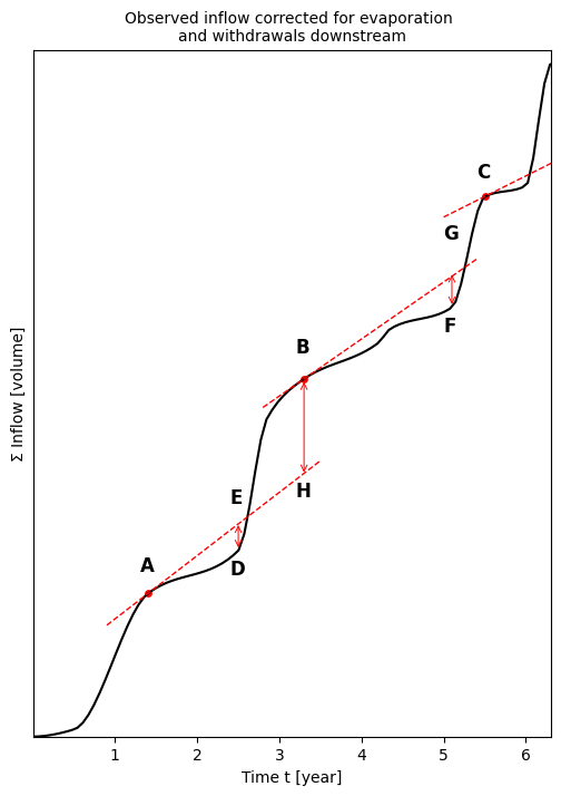
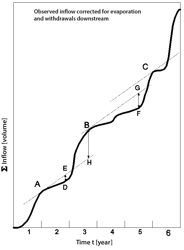
Fig. 2.9 Summation curve of inflow, also known as the Rippl diagram.

It is also possible that the demand is not constant, and there is a need to provide for variable water supply; the demand line becomes a curve, but the analysis remains the same. In this case, it is crucial that the demand curve corresponds chronologically to the summation curve, meaning only vertical displacement occurs.

A summation curve can also be used to determine the expected water supply for a given capacity; the demand lines are drawn in a way that the maximum distance to the summation curve does not exceed the given capacity. The slopes of the demand lines then indicate the maximum delivery in each period. One condition is that a demand line must intersect the summation curve when extended; if this is not the case, the reservoir will not be filled anymore.

The operation of a reservoir in a specific period can be monitored by plotting summation curves, as shown in Fig. 2.10.

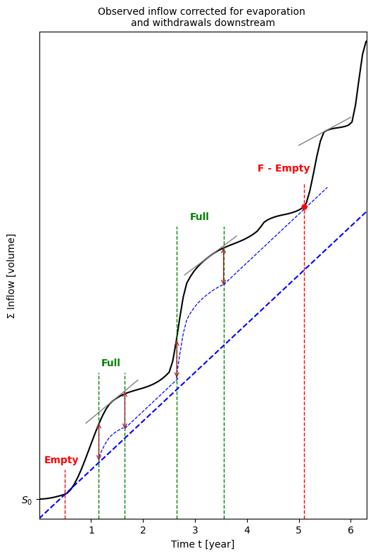
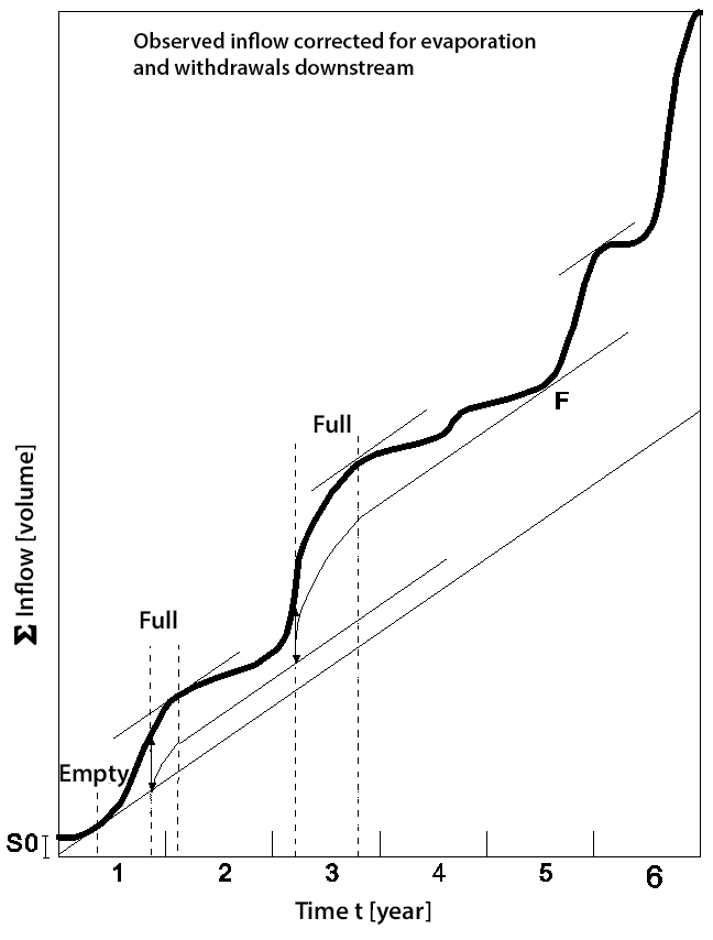
Fig. 2.10 Operation of a reservoir monitored using summation curves.

At the beginning of the first year, an initial stock storage \(S_0\) is required, allowing the reservoir level to decrease to \(0\) after a few months. Due to the subsequent large inflow, the reservoir becomes full; the arrow corresponds to distance \(FG\) from Fig. 2.9. From this moment until the time when the delivery exceeds the inflow again, water will be discharged through the emergency spillway. Therefore, the vertical distance between inflow and total outflow remains unchanged as long as the reservoir is full. Afterwards, a period of water withdrawal follows, which subsequently is followed by a period of refilling until the reservoir capacity is reached again. Fig. 2.9 shows that the reservoir is precisely empty at point F; this is correct because the capacity was calculated based on the difference between demand and inflow at this point.

2.4.4.2. Computer simulations for capacity determination

Another way to determine the required capacity for a reservoir is by using computer simulations. Simulations utilize historical or artificially generated time series for inflow. For each time step, a water balance is determined for all inflowing water and the water leaving the reservoir. The advantage is that outgoing terms such as evaporation, leakage, and water flowing over the emergency spillway can be made dependent on the actual storage. For open water evaporation, the reservoir surface area is essential, related to the storage via the capacity curve. One can also choose to make evaporation dependent on weather parameters. With a specific demand pattern for water from the reservoir, the capacity can be chosen such as to meet the expectations, allowing for a certain percentage of the time not meeting the demand. For example, for reservoirs supplying irrigation water a relatively higher failure percentage may be acceptable compared to drinking water reservoirs. The advantage of a higher failure probability is that a considerably cheaper reservoir can often be constructed due to the smaller required capacity.

At each time step \(\Delta t\), the storage is determined as follows:

(2.16)\[ S_\text{2} = S_\text{1} + I \Delta t -(O + E_\text{o} + L)\Delta t - N \Delta t \quad \text{[L$^{3}$]} \]

where:

\(I\)	influx	[L\(^{3}\)/T]
\(O\)	outflux	[L\(^{3}\)/T]
\(E_\text{o}\)	open water evaporation	[L\(^{3}\)/T]
\(L\)	leakage	[L\(^{3}\)/T]
\(N\)	spillage	[L\(^{3}\)/T]
\(S_\text{1}\)	volume at t=1	\([\mathrm{L}^{3}]\)
\(S_\text{2}\)	volume at t=2	\([\mathrm{L}^{3}]\)

Subject to the condition that \(S_\text{2} > 0\) and \(S_\text{2} \leq S_\text{max}\). In case \(S_\text{2} < 0\), the demand \(O\) needs to be reduced. In case \(S_2 > S_\text{max}\), a certain amount of water (\(N\)) will flow over the spillway. Conveniently, \(N\) is often determined such that \(S_\text{2} = S_\text{max}\). If \(S_\text{2} \leq S_\text{max}\), then \(N=0\) obviously applies. For a more detailed explanation of this method, see the example below.

2.4.4.3. Other factors

Before a decision can be made about the capacity of a reservoir, a detailed study is usually conducted for one or more periods for which data is available. This involves investigating what the leakage losses are as a function of the water level. Additionally, evaporation is related to the water surface of the reservoir. Operational strategies can be tested for their feasibility using computers.

# Note that the code cells below is used for the website only.

Exercise 2.3

From a natural reservoir built in a river, the inflow is provided for an average year and per month, starting from the beginning of the wet season (see the table below). For all questions, we assume that the reservoir is empty at the beginning of the wet season. The withdrawals requested include evaporation and leakage losses. We calculate only based on effective storage.

Table 2.2 Reservoir data

Month	Influx [\(\cdot 10^6\) \(\text{m}^3 \over \text{month}\)]
Oct	30
Nov	40
Dec	60
Jan	50
Feb	20
Mar	15
Apr	10
May	10
Jun	5
Jul	0
Aug	0
Sep	0

a) What can be the maximum constant withdrawal during the average year?

b) What should be the minimum effective storage of the reservoir for this calculated constant withdrawal?

We now assume there is no withdrawal during the first four months.

c) What is the maximum constant withdrawal for the remaining part of the year now?

d) What is now the minimum effective storage to meet this maximum constant withdrawal, considering no withdrawals during the first four months?

In the months between October and January, there is again no withdrawal. After that, the maximum withdrawal is \(30 \cdot 10^6\) \(\text{m}^3 \over \text{month}\). The effective storage of the reservoir is \(100 \cdot 10^6\) \(\text{m}^3\). When the effective storage of the reservoir is exceeded, the surplus will flow from the reservoir over a spillway.

e) What are the monthly withdrawals (withdrawal + spillway) now?

Answer Exercise 2.3a

\[ \sum \text{Influx} = 240 \cdot 10^6 \frac{\text{m}^3}{\text{month}} \]

\[ \text{Withdrawal} = \frac{\sum \text{Influx}}{12 \text{months}} = 20 \cdot 10^6 \frac{\text{m}^3}{\text{month}} \]

Answer Exercise 2.3b

We need to calculate how much water there is inside the reservoir during the year using Equation (2.16). In the months of Januray and February the reservoir is at its fullest, the volume of which should be equal to the minimum effective storage size.

Table 2.3 part_b

Month	Volume of water in the reservoir [\(\cdot 10^6\) \(\text{m}^3\)]
Oct	0 + 30 - 20 = 10
Nov	10 + 40 - 20 = 30
Dec	30 + 60 - 20 = 70
Jan	70 + 50 - 20 = 100
Feb	100 + 20 - 20 = 100
Mar	100 + 15 - 20 = 95
Apr	95 + 10 - 20 = 85
May	85 + 10 - 20 = 75
Jun	75 + 5 - 20 = 60
Jul	60 + 0 - 20 = 40
Aug	40 + 0 - 20 = 20
Sep	20 + 0 - 20 = 0

Answer Exercise 2.3c

During the first four months there is no withdrawal so there is \(4 \cdot 20 \cdot 10^6 \: \text{m}^3 = 80\) \(\cdot 10^6\) \(\text{m}^3\) extra to withdraw during the last eight months.

Withdrawal during the last eight months is therefor

\[ \text{Withdrawal} = 20 \cdot 10^6 \frac{\text{m}^3}{\text{month}} + \frac{80 \: \text{m}^3}{8 \: \text{months}} = 30 \cdot 10^6 \frac{\text{m}^3}{\text{month}} \]

Answer Exercise 2.3d

Since there is no withdrawal during the first four months, the volume of water in the reservoir is simply equal to the total influx. The largest amount of volume in the reservoir is now in Januray with \(180 \cdot 10^6\) \(\text{m}^3\):

Table 2.4 part_d

Month	Volume of water in the reservoir [\(\cdot 10^6\) \(\text{m}^3\)]
Oct	0 + 30 = 30
Nov	30 + 40 = 70
Dec	70 + 60 = 130
Jan	130 + 50 = 180
Feb	180 + 20 - 30 = 170
Mar	170 + 15 - 30 = 155
Apr	155 + 10 - 30 = 135
May	135 + 10 - 30 = 115
Jun	115 + 5 - 30 = 90
Jul	90 + 0 - 30 = 60
Aug	60 + 0 - 30 = 30
Sep	30 + 0 - 30 = 0

Answer Exercise 2.3e

Since there is no withdrawal during the first four months, the volume of water in the reservoir is simply equal to the total influx. The largest amount of volume in the reservoir is now in Januray with \(180 \cdot 10^6\) \(\text{m}^3\):

Table 2.5 part_e

Month	Volume of water in the reservoir [\(\cdot 10^6\) \(\text{m}^3\)]
Oct	0 + 30 - 0 = 30
Nov	30 + 40 - 0 = 70
Dec	70 + 60 - 0 - 30 = 100
Jan	100 + 50 - 0 - 50 = 100
Feb	100 + 20 - 30 = 90
Mar	90 + 15 - 30 = 75
Apr	75 + 10 - 30 = 55
May	55 + 10 - 30 = 35
Jun	35 + 5 - 30 = 10
Jul	10 + 0 - 10 = 0
Aug	0 + 0 - 30 = 0
Sep	0 + 0 - 30 = 0

# Note that the code cells below is used for the website only.

Exercise 2.4

Let us consider a reservoir with a maximum storage of \(S_\text{max} = 80\) \(\cdot 10^6\) \(\text{m}^3\). The reservoir owners desire a water supply of \(O_\text{des} = 25\) \(\cdot 10^6\) \(\text{m}^3 \over \text{month}\). Lastly, the reservoir is initially empty.

a) Over a 24-month period the influx into the reservoir and the amount of water stored in the reservoir are measured. However, some of the data has gone missing. Using equation (2.16), find the missing data for December and March.

b) The reservoir owners are frustrated they could not consistently withdraw the desired amount during the 24-month period. They ask you if by increasing the storage size of the reservoir, they could have consistently withdrawn the desired amount. Using the graph below, determine if that would have been possible, and if so, what storage capacity would have been sufficient?

Table 2.6 Rippl reservoir data

Month	Influx [\(\cdot 10^6\) \(\text{m}^3 \over \text{month}\)]	Desired withdrawal [\(\cdot 10^6\) \(\text{m}^3 \over \text{month}\)]	Actual withdrawal [\(\cdot 10^6\) \(\text{m}^3 \over \text{month}\)]	Spillage [\(\cdot 10^6\) \(\text{m}^3 \over \text{month}\)]	Storage [\(\cdot 10^6\) \(\text{m}^3\)]
					0
Oct	25	25	25	0	0
Nov	30	25	25	0	5
Dec	35	25	25	0	?
Jan	50	25	25	0	40
Feb	80	25	25	15	80
Mar	40	25	25	?	80
Apr	20	25	25	0	75
May	15	25	25	0	65
Jun	15	25	25	0	55
Jul	10	25	25	0	40
Aug	5	25	25	0	20
Sep	0	25	20	0	0
Oct	0	25	0	0	0
Nov	15	25	15	0	0
Dec	20	25	20	0	0
Jan	25	25	25	0	0
Feb	50	25	25	0	25
Mar	60	25	25	0	60
Apr	80	25	25	35	80
May	15	25	25	0	70
Jun	15	25	25	0	60
Jul	5	25	25	0	40
Aug	5	25	25	0	20
Sep	5	25	25	0	0

Answer Exercise 2.4a

Determining the storage level in December is performed simply using Equation (2.16):

\[ S_2 = 5 + 35 - 25 = 15 \: \cdot 10^6 \frac{\text{m}^3}{\text{month}} \]

To calculate the spillage in March we also use Equation (2.16). If we find that the new level of storage \(S_2\) exceeds the maximum storage \(S_{max}\), the excess of storage will become spillage.

\[ S_2 = 80 + 40 - 25 = 95 \: \cdot 10^6 \frac{\text{m}^3}{\text{month}} \]

which exceeds the maximum storage level of \(S_{max} = 80\) \(\cdot 10^6\) \(\text{m}^3\) by \(15\) \(\cdot 10^6\) \(\text{m}^3\). Therefore, the spillage for March is \(15\) \(\cdot 10^6\) \(\text{m}^3\).

Below, the Rippl diagram describes the storage in the reservoir. The code performs the same calculation as you have made by hand above, and outputs the cumulative influx and outflux to easily plot the Rippl diagram.

Show code cell content Hide code cell content

import numpy as np
import pandas as pd
import matplotlib.pyplot as plt

%matplotlib widget

plt.rcParams.update({'font.size': 12, 'lines.linewidth': 2})

influx = np.array([25, 30, 35, 50, 80, 40, 20, 15, 15, 10, 5, 0, 0, 15, 20, 25, 50, 60, 80, 15, 15, 5, 5, 5])

def rippl(influx, desired_outflux, initial_storage, maximum_storage):

    # Create a DataFrame to store the simulation results
    d = {
        'Influx': influx,
        'Desired withdrawal': desired_outflux * np.ones(len(influx)),
        'Real withdrawal': np.nan * np.ones(len(influx)),
        'Spillway': np.nan * np.ones(len(influx)),
        'Storage': np.nan * np.ones(len(influx))
    }
    df = pd.DataFrame(data=d)

    # Initialize the current storage
    current_storage = initial_storage

    # Simulate water inflow, outflow, and storage for each month
    for i in range(len(influx)):
        flux_in = df.loc[i, 'Influx']
        flux_out_desired = df.loc[i, 'Desired withdrawal']

        # Check if there's not enough water for the desired withdrawal
        if current_storage + flux_in < flux_out_desired:
            df.loc[i, 'Real withdrawal'] = current_storage + flux_in
            df.loc[i, 'Spillway'] = 0
        
        # Check if there's too much water and limit the withdrawal
        elif current_storage + flux_in - flux_out_desired > maximum_storage:
            df.loc[i, 'Real withdrawal'] = flux_out_desired
            df.loc[i, 'Spillway'] = current_storage + flux_in - flux_out_desired - maximum_storage
        
        # There isn't too much or too little water, so withdraw the desired amount
        else:
            df.loc[i, 'Real withdrawal'] = flux_out_desired
            df.loc[i, 'Spillway'] = 0

        # Calculate the new storage level
        new_storage = current_storage + flux_in - df.loc[i, 'Real withdrawal'] - df.loc[i, 'Spillway']
        df.loc[i, 'Storage'] = new_storage

        # Update the current storage for the next iteration
        current_storage = new_storage

    # Calculate the cumulative water influx and outflux
    df['Cumulative influx'] = df['Influx'].cumsum()
    df['Cumulative outflux'] = df['Real withdrawal'].cumsum() + df['Spillway'].cumsum()

    return df['Cumulative influx'].values, df['Cumulative outflux'].values

res = rippl(influx, 25, 0, 80)

plt.figure()
# Plot the cumulative influx and outflux as a rippl diagram
plt.plot(np.arange(1, len(influx) + 1), res[0], '.-', label = "Cumulative influx")
plt.plot(np.arange(1, len(influx) + 1), res[1], '.-', label = "Cumulative outlfux")
plt.xlabel('Month number')
plt.ylabel('Volume [$\cdot 10^6$ m$^3$]')
plt.title('Rippl diagram')
plt.grid()
plt.legend()

plt.show()

<>:66: SyntaxWarning:

invalid escape sequence '\c'

<>:66: SyntaxWarning:

invalid escape sequence '\c'

/tmp/ipykernel_133/4118848130.py:66: SyntaxWarning:

invalid escape sequence '\c'

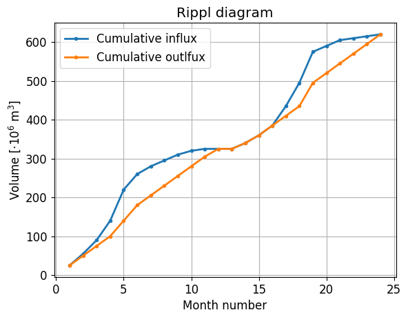
Answer Exercise 2.4b

In the Rippl diagram, the amount of storage in the reservoir is characterized by the difference between the cumulative influx and the cumulative outflux. By moving the slider under the graph (hence changing the storage size) it can be noticed that the cumulative outflux becomes less steep around month 13, even for large storage sizes. This means that the cumulative influx up until month 13 is insufficient to deliver the desired withdrawal up until that point.

2.4.5. Reservoirs for flood control

A reservoir can also serve to partially capture high flows, reducing the risk of flooding. The principle behind this is to distribute the discharge wave over a longer period, so that the water is discharged with a delay and a lower maximum flow rate. In this case, determining the reservoir capacity is not about the maximum flow rate, but rather the amount of water that enters within a certain time. A reservoir that is specifically built to dampen high flow peaks is called a retention reservoir; a reservoir built for a different purpose can also be used for flood control. A simple representation of how a retention reservoir works is as follows: as a high flood wave approaches, the discharge outlets of the reservoir are fully opened. This maximizes the storage capacity before the high flood wave reaches the reservoir. By doing so, the activation of the emergency overflow is prevented or delayed for as long as possible when the high flood wave enters. In the case of a fixed outflow opening, the relationship between water level and discharge is important. If this relationship is known, the outflow can be calculated for a given inflow, providing insight into the usefulness of a reservoir for flood control.

2.4.6. Effects of a reservoir

The construction and operation of a reservoir usually results in significant changes in the surrounding environment. A reservoir requires a lot of space, which comes at the expense of the original functions of an area. As long as it concerns economic activities, the loss of space can be quantified to some extent in terms of money; however, factors like emotional values, landscape, and natural values also come into play. Such factors are difficult to express in monetary terms or quantify in other ways. Therefore, a sophisticated balance must always be considered between the advantages and disadvantages of building a reservoir, no matter how subjective these pros and cons may be. The intended function of a reservoir can play a crucial role in such considerations. For instance, if a certain area frequently experiences flooding due to high flood peaks, that area incurs damage as a result. If the damage caused by the construction of a retention reservoir is deemed to be less than the flood damage, the decision seems obvious. Nevertheless, the consideration remains highly complex in such cases because not all effects of reservoir construction can be predicted, and the proper functioning cannot be guaranteed with 100% certainty.

Aswan Dam

In the Nile, the Aswan Dam has been constructed to create a reservoir that significantly increases irrigation potential along the Nile. However, the construction of the Aswan Dam has also led to a reduction in the amount of sediment the Nile carries to the Mediterranean Sea, causing significant changes in the Nile Delta; measures now need to be taken to combat coastal erosion. Additionally, the increased irrigation has resulted in the spread of the disease schistosomiasis over a wide area through the irrigation water.

2.4.7. Water storage in The Netherlands

As mentioned in Chapter 3 Hydrology of the Netherlands, in The Netherlands we also deal with water storage, but in a somewhat different form than in mountainous regions. In a flat country like The Netherlands, extensive and relatively shallow waters serve as reservoirs. With the construction of the Afsluitdijk and the Delta Works, large reservoirs have been created that contribute to the management of water resources in The Netherlands. This allows the water system to be adapted as effectively as possible to the various functions that water serves. Since these reservoirs have emerged primarily as a result of measures aimed at safety, they do not have just a single function; the northern delta basin for instance serves not only for freshwater supply, but as a buffer against salinity as well. Additionally, this basin has enabled a portion of the Rhine water to be used to meet the increasing water needs in the areas around the IJsselmeer and to make the IJssel River more navigable.

Moreover, one of the reservoir functions of the IJsselmeer is for example the storage of excess precipitation during the winter period to meet the water demand for agriculture in the summer. To achieve this, specific water levels, known as target levels (NL: streefpeilen), are maintained in the IJsselmeer through the management of the sluices in the Afsluitdijk. Furthermore, there are numerous polders in The Netherlands where the ditches (NL: sloten) also serve a distinct reservoir function. For each polder, a target level, called the polder level (NL: polderpeil), is established. By allowing water to flow in or out from the ditches, this level can be maintained as effectively as possible.