GPs for Regression

In order to use Gaussian Processes for regression, the first step is of course to observe some targets \(\mbf{t}\). We again assume an observation model of the form:

(77)\[ p(t\vert y) = \mathcal{N}\left(t\vert y(\mathbf{x}),\beta^{-1}\right) \]

which means that we observe \(y\) only indirectly, polluted by a Gaussian noise with variance \(\beta^{-1}\). With the usual i.i.d. assumption, we get that conditioned on \(y\), individual target observations are independent from each other (conditional independence).

Furthermore, we would also like to predict a new target value \(\hat{t}\). With all this new information, we can adapt our graph model from before:

Fig. 30 A GP graph but now with noisy target observations and prediction for \(y\) at a new input \(\hat{\bx}\).

and following the joint distribution encoded by the graph (check this by hand!), we can arrive at a marginal for all our \(N\) targets \(\mbf{t}\) at (stacked) inputs \(\mbf{X}\):

(78)\[ p(\mbf{t}) = \displaystyle\int p(\mbf{t}\vert\mbf{y})p(\mbf{y})\,\mrm{d}\mbf{y} = \gauss\left(\mbf{t}\vert\mbf{0},K(\mbf{X},\mbf{X}) + \beta^{-1}\mbf{I}\right) \]

where we once again have simply followed the standard result for a Gaussian marginal under Bayesian inversion, in this case with \(\bs{\Sigma} = K(\mbf{X},\mbf{X})\), \(\mbf{A}=\mbf{I}\) and \(\mbf{L}^{-1}=\beta^{-1}\mbf{I}\).

From Eq. (76) we have seen previously, we can now easily include \(\hat{t}\) in the joint:

(79)\[\begin{split} p(\mbf{t},\cB{\hat{t}}) = \gauss\left( \mbf{t},\cB{\hat{t}}\left\vert\right.\mbf{0}, \begin{bmatrix} K\left(\mbf{X},\mbf{X}\right) + \beta^{-1}\mbf{I} & \cE{K\left(\mbf{X},\hat{\bx}\right)} \\ \cA{K\left(\hat{\bx},\mbf{X}\right)} & \cB{k\left(\hat{\bx},\hat{\bx}\right)} + \beta^{-1} \end{bmatrix} \right) \end{split}\]

where you should pay special attention to what comes from \(p(\mbf{y})\) and what comes from the observation model, namely the noise \(\beta\). Finally, again using the standard result for multivariate Gaussians, we can condition \(\hat{t}\) on \(\mbf{t}\) and reach our posterior predictive distribution:

(80)\[ p(\hat{t}\vert\mbf{t}) = \gauss\left( \hat{t}\vert \hat{m},\hat{\sigma}^2 \right) \]

with posterior mean:

(81)\[ \hat{m} = \cA{K\left(\hat{\bx},\mbf{X}\right)} \left[ K\left(\mbf{X},\mbf{X}\right) + \beta^{-1}\mbf{I} \right]^{-1} \mbf{t} \]

and posterior variance:

(82)\[ \hat{\sigma}^2 = \cB{k\left(\hat{\bx},\hat{\bx}\right)} - \cA{K\left(\hat{\bx},\mbf{X}\right)} \left[ K\left(\mbf{X},\mbf{X}\right) + \beta^{-1}\mbf{I} \right]^{-1} \cE{K\left(\mbf{X},\hat{\bx}\right)} + \beta^{-1} \]

and we can just as easily predict for multiple values of \(\hat{t}\) at once by using a block \(\hat{\bx}\), in which case the mean becomes a vector and the variance becomes a covariance matrix.

Look again at the expressions above: note how a GP for regression is a non-parametric model. Instead of storing information obtained during training in a weight vector, we always need the values of \(\mbf{t}\) and \(\mbf{X}\) to make new predictions.

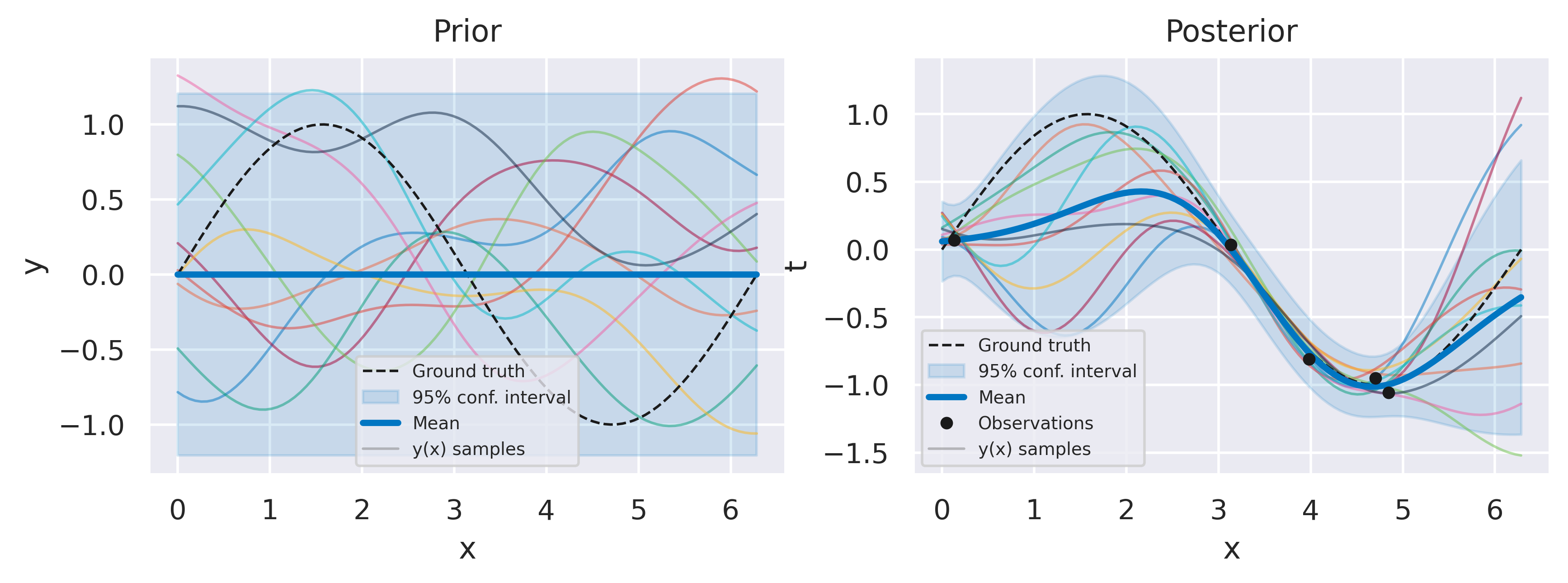
Below you can see an example of GP model for regression for a one-dimensional input. We opt for a Squared Exponential kernel. On the left you can see the prior over \(t\) (mean and two standard deviations) with draws from \(y(x)\) also shown. On the right you can see the posterior over \(\hat{t}\) for the whole domain including some draws from the posterior over functions \(p(\mbf{y}\vert\mbf{t})\).

Fig. 31 Example of GP for regression, prior (left) and posterior (right) over \(t\), with ten function draws from \(y(x)\) in each plot.

Note how all desirable features for a robust model are present:

• The model avoids overfitting even for very small datasets;

• Mean and sampled functions fit closely to the observed data;

• The variance gives a measure of prediction uncertainty, increasing away from the observations;

• Hyperparameters are learned directly from data without the need for a validation dataset.

In the next page we will go through this last point, namely how to determine suitable values for the kernel hyperparameters.