From Weights to Functions#
For this part of the course we keep working with the familiar basis function models we have been using:
where for regression problems we would use it directly together with some observation noise to define our targets, while in classification we would first feed it into a logistic sigmoid before using it.
For now let us leave the application aside and just assume we have a vector with values of \(y(\bx)\) for several \(\bx\). Using the expression above and defining \(\Basis_{nk}=\basis_k(\bx_n)\) we have:
and since \(p(\bw)=\mathcal{N}(\mbf{0},\alpha^{-1}\mbf{I})\) and we can therefore grab as many samples of \(\bw\) from our bag as we want, that means \(\mbf{y}\) is also jointly Gaussian:
where you can see that \(\bw\) vanished, and we can instead just sample from \(\mbf{y}\) instead of \(\bw\)!
Further Reading
If you are interested in the exact derivation of going from \(\bw\) to \(\mbf{y}\), read Section 6.1 and the beginning of 6.4.1.
bishop-prml
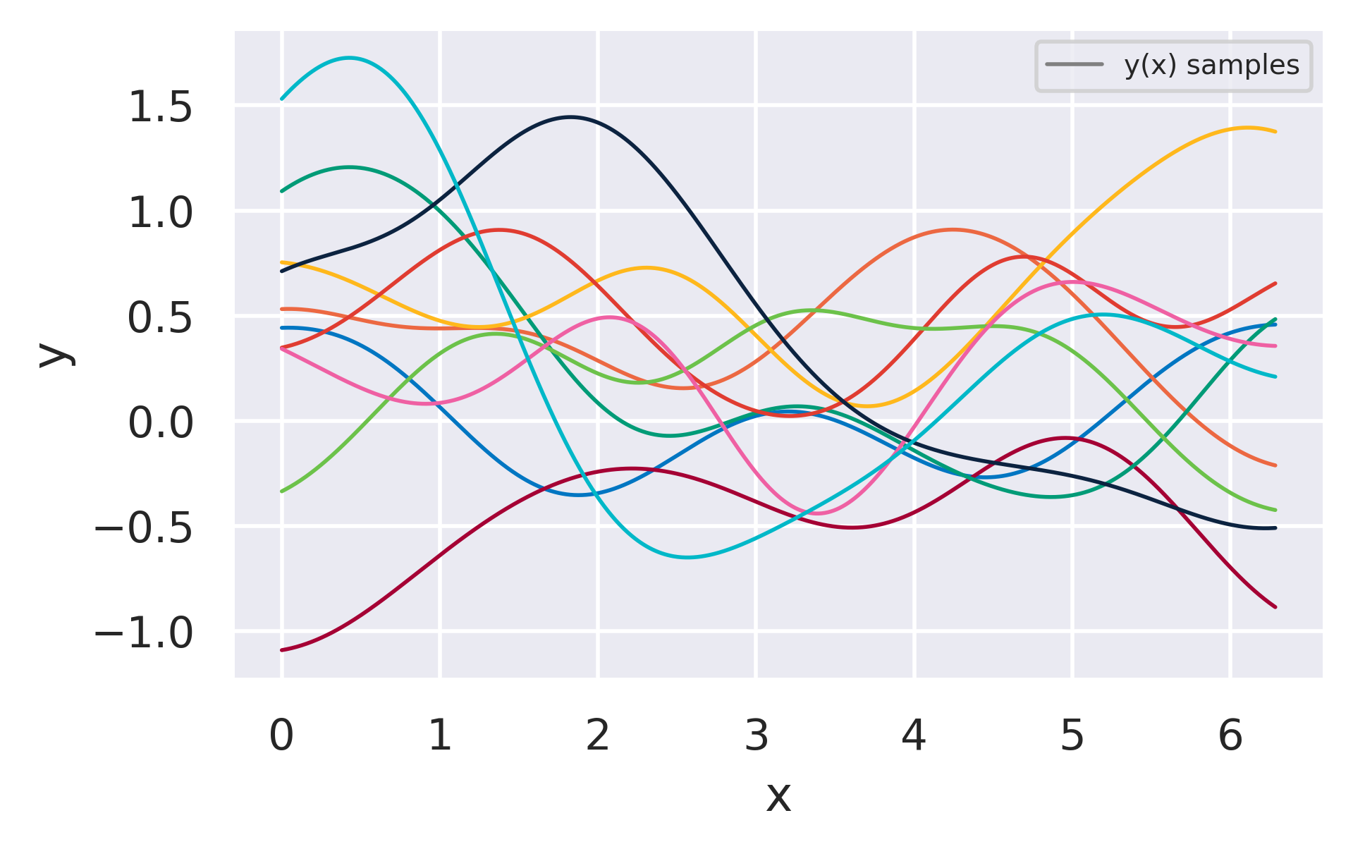
We have actually already seen an example of this before when looking at Active Learning. For a set of radial basis functions and sampling from the prior over \(\bw\) we got the following samples:

Fig. 26 Samples from a basis function model obtained by sampling from the prior \(p(\bw)\) and plotting the resulting \(y(x)\). The same curves could also have been directly sampled from \(p(\mbf{y})\) instead.#
If we instead sampled from Eq. (70) we would get very similar curves. But how does one sample a function? That might feel a bit weird, but it is actually straightforward: each curve above is composed of 1000 \(y\) values for different \(x\). To get one of them we just need to compute the \(1000\times 1000\) matrix \(\mbf{K}\) and sample from the size-1000 version of Eq. (70).
Each entry in \(\mbf{K}\) relates two different values of \(\bx\). We can write one of these entries as:
and we call \(k(\bx_m,\bx_n)\) a kernel function.
