Gaussian Processes#
In the previous page we have found a way to convert a model based on weights \(\bw\) to an exactly equivalent model based on functions represented by multivariate Gaussian distributions with a covariance matrix based on a kernel function. The model we just saw is an example of a Gaussian Process, which we now define formally:
Gaussian Process (GP)
A Gaussian probability density over functions. In practice, this manifests as any arbitrary number of points in the function being jointly Gaussian.
Just as in any Gaussian, a GP can be fully described by its mean and covariance:
where \(m(\bx)\) is a mean function and \(k(\bx,\bx')\) is a kernel that defines the covariance between any two points \(\bx\) and \(\bx'\).
We can represent any number of values of \(y(\bx)\) as a probabilistic graph, as we have been doing. Because every value of \(y\) is correlated with every other value (through the covariance \(\mbf{K}\)), we can draw a few graphs as below:
Fig. 27 Examples of graphs with two, three or four fully-connected jointly-Gaussian \(\mbf{y}\) values.#
The joint densities for each of the three graphs above would be, respectively:
Looking at the equations above, the pattern shoud become quite clear. Due to the simple marginalization result for Gaussian densities, any number of variables in the process can be described by themselves or in blocks. Adding a new variable to the mix simply means adding the colored submatrices you see above. Note also that the blue and yellow parts are the transpose of each other since Gaussians have symmetric covariances.
Since this leads to a fully connected set of an arbitrary number of \(\mbf{y}\) nodes, we generalize the graphs above:
Fig. 28 Generalization of the previous graphs, now representing a Gaussian Process with an arbitrary number \(N\) of values of function \(y(\bx)\).#
where the arrows connecting the \(y\) nodes have been changed to a thick line that represents full connectivity. Finally, becasue this graph has an arbitrary number of nodes, we can further simplify it to:
Fig. 29 Graph representation of a GP prior, with \(N\) jointly Gaussian values of \(y(\bx)\).#
which is the graph representing the prior over \(y(\bx)\), since nothing is observed yet. We will take care of that soon. Considering a prior with \(m(\bx)=0\) for simplicity (recall this is equivalent to a prior over \(\bw\) with zero mean), we can get to a general expression for the joint over two groups of function values \(\mbf{y}_a\) and \(\mbf{y}_b\):
where \(\mbf{X}\) represents a stacking of \(\bx\) values and \(K\) is the matrix version of \(k(\bx,\bx')\).
Kernel engineering#
For basis function models we had \(m(\bx)=\mbf{0}\) and \(k(\bx,\bx')=\frac{1}{\alpha}\basis(\bx)^\T\basis(\bx')\). But why stop there? We can also make our own kernels, as long as the covariance for any set of function values is positive definite. This is called kernel engineering. Discovering new kernels with good properties for specific applications is an active field of research.
A very popular choice of kernel is the so-called squared exponential:
where \(\sigma_f\) is a scaling factor and \(\ell\) is a length scale that controls the correlation between function values.
The kernel above is infinitely differentiable, and that is not always a desirable property. Another popular kernel that addresses this issue is the Matérn kernel:
where \(\nu\) controls the degree of differentiability of the functions drawn from the kernel, \(\Gamma(\cdot)\) is the Gamma function and \(K_\nu(\cdot)\) is a Modified Bessel function.
Click through the tabs below to have a feeling for different kernels. On the left you see a graphical representation of the covariance \(\mbf{K}\), with darker tones representing lower values and lighter tones higher values. On the right you see samples of the function \(y(x)\) drawn from Eq. (72) with \(m(x)=0\) and different kernels. Again note that we do not really sample a function from the process but simply pick 100 values of \(x\) in our range of interest, assemble a covariance \(\mbf{K}\) with entries given by the kernel and sample from the joint \(p(\mbf{y}\vert\mbf{0},\mbf{K})\).
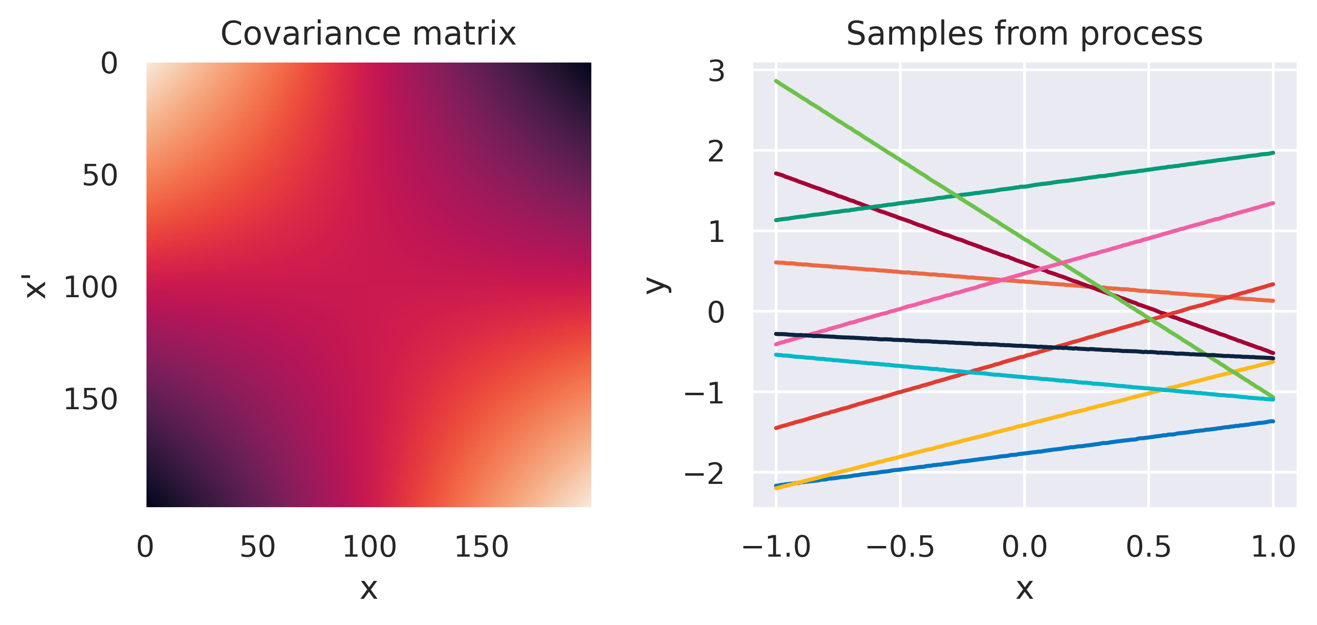
\(k(\bx,\bx') = \displaystyle\frac{1}{\alpha}\basis(\bx)^\T\basis(\bx')\)
\(\phi_m = x^m\)
\(\color{red}m = \left\{0,1\right\}\)
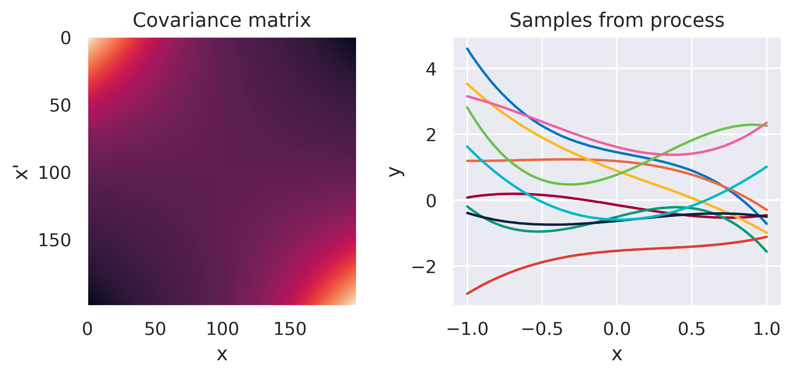
\(k(\bx,\bx') = \displaystyle\frac{1}{\alpha}\basis(\bx)^\T\basis(\bx')\)
\(\phi_m = x^m\)
\(\color{red}m = \left\{0,\dots,3\right\}\)
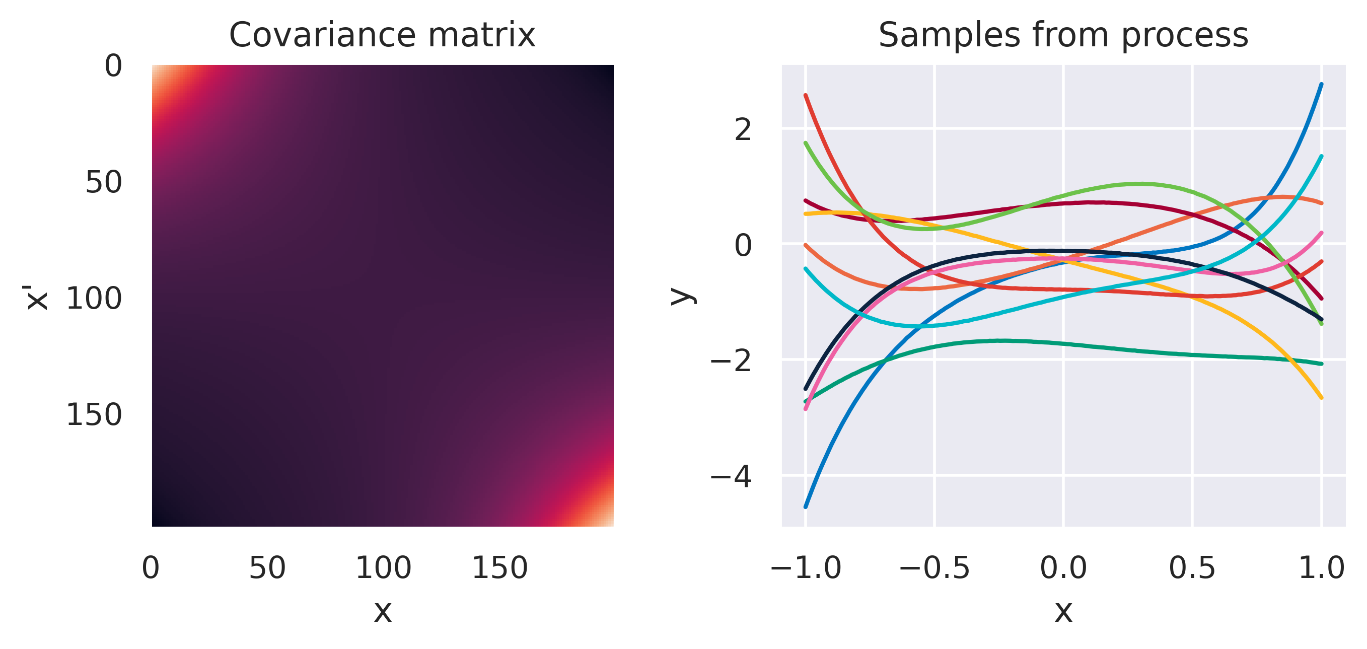
\(k(\bx,\bx') = \displaystyle\frac{1}{\alpha}\basis(\bx)^\T\basis(\bx')\)
\(\phi_m = x^m\)
\(\color{red}m = \left\{0,\dots,5\right\}\)
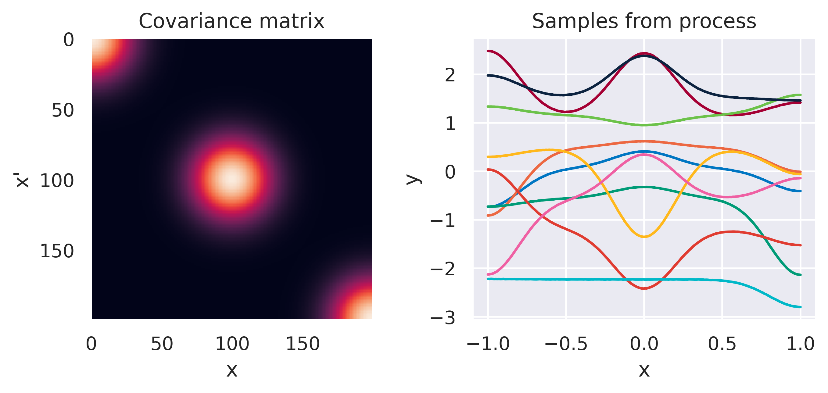
\(k(\bx,\bx') = \displaystyle\frac{1}{\alpha}\basis(\bx)^\T\basis(\bx')\)
\(\phi_m=\exp\left[\displaystyle\frac{(x-\mu_m)^2}{2s_m^2}\right]\)
\(\color{red}M=3\), \(s=0.2\)
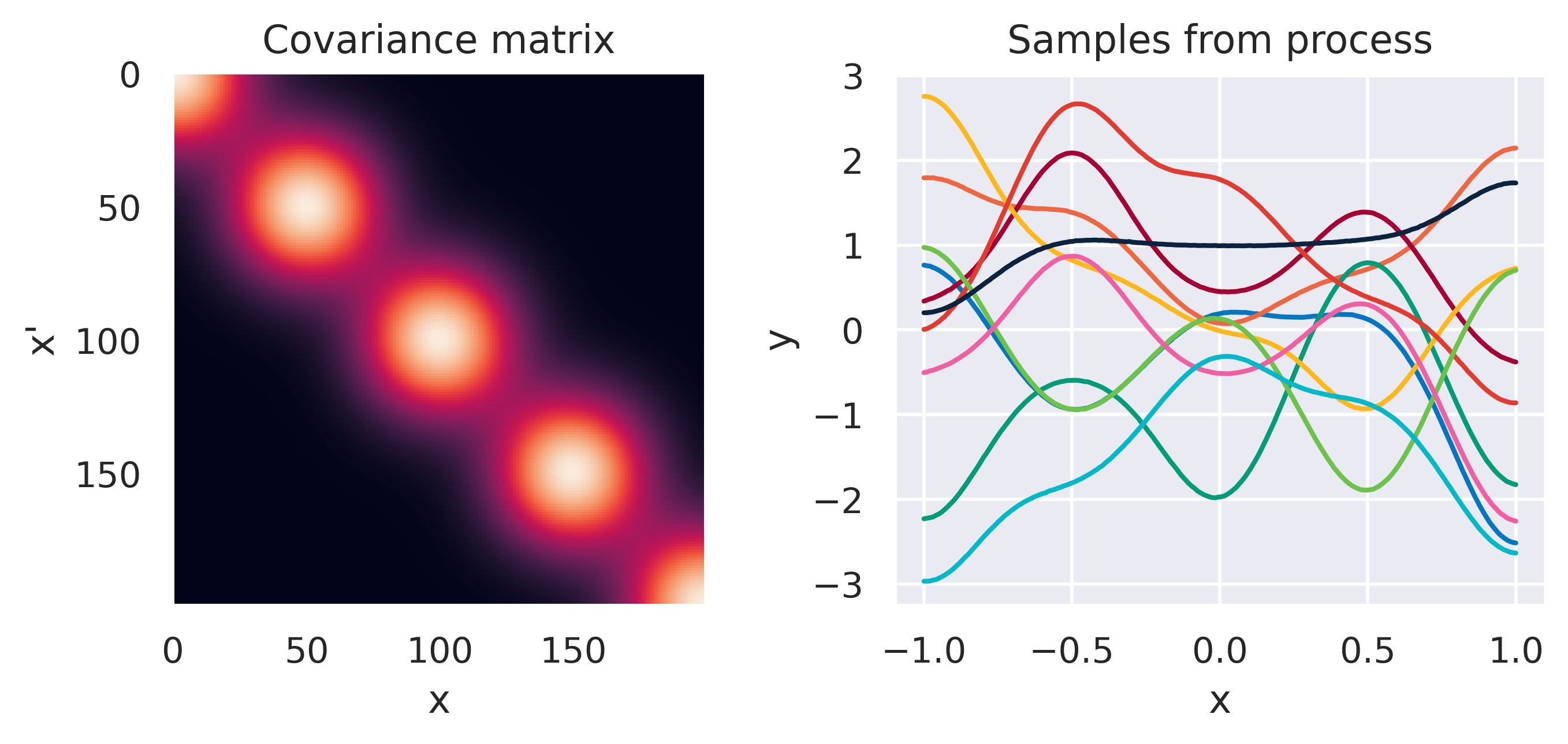
\(k(\bx,\bx') = \displaystyle\frac{1}{\alpha}\basis(\bx)^\T\basis(\bx')\)
\(\phi_m=\exp\left[\displaystyle\frac{(x-\mu_m)^2}{2s_m^2}\right]\)
\(\color{red}M=5\), \(s=0.2\)
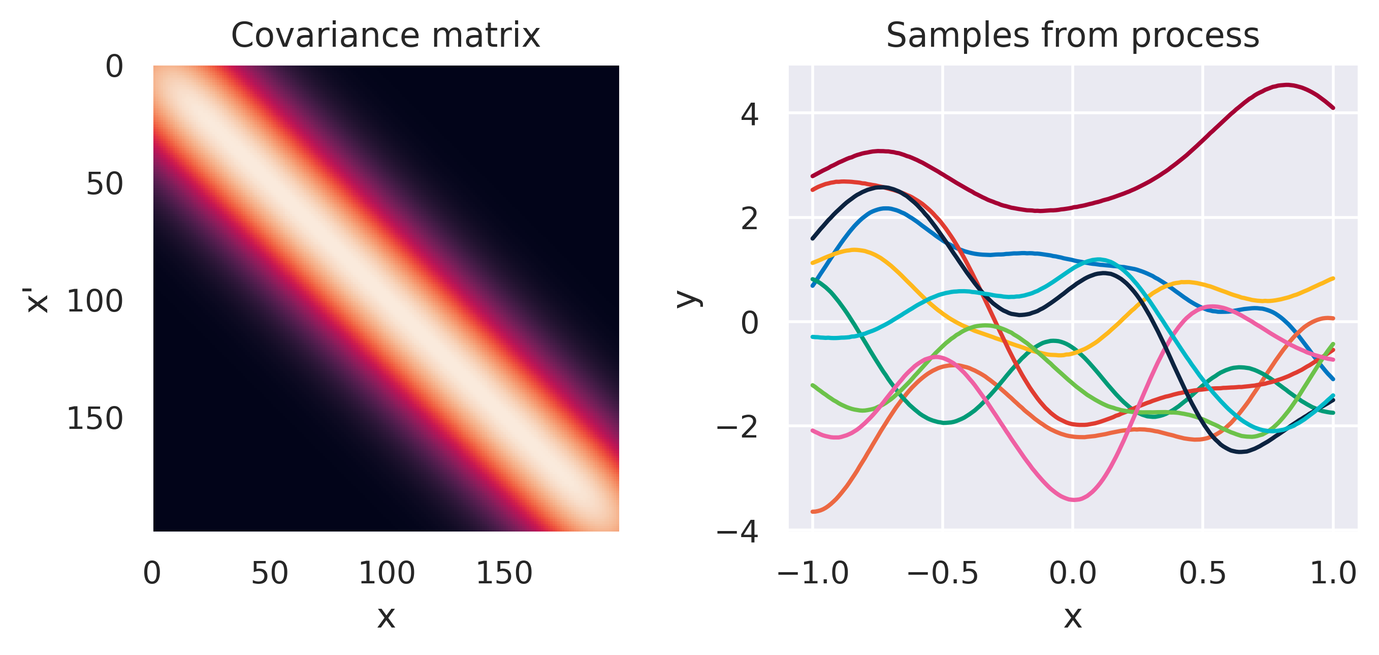
\(k(\bx,\bx') = \displaystyle\frac{1}{\alpha}\basis(\bx)^\T\basis(\bx')\)
\(\phi_m=\exp\left[\displaystyle\frac{(x-\mu_m)^2}{2s_m^2}\right]\)
\(\color{red}M=10\), \(s=0.2\)
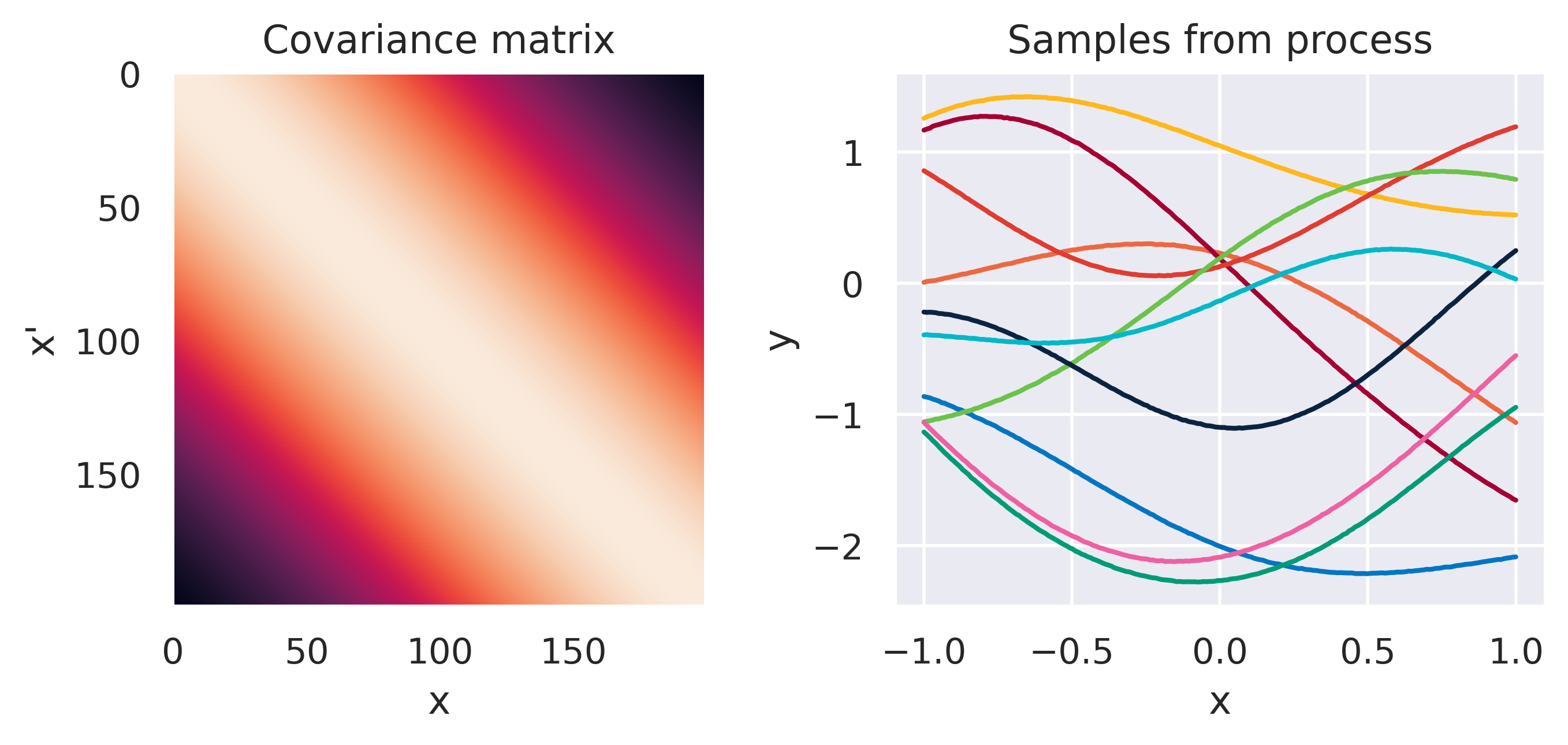
\(k(\bx,\bx') = \sigma_f^2\exp\left(\displaystyle-\frac{d^2}{2\ell^2}\right)\)
\(d = \lVert\bx-\bx'\rVert\)
\(\sigma_f=1\), \(\color{red}\ell=1\)
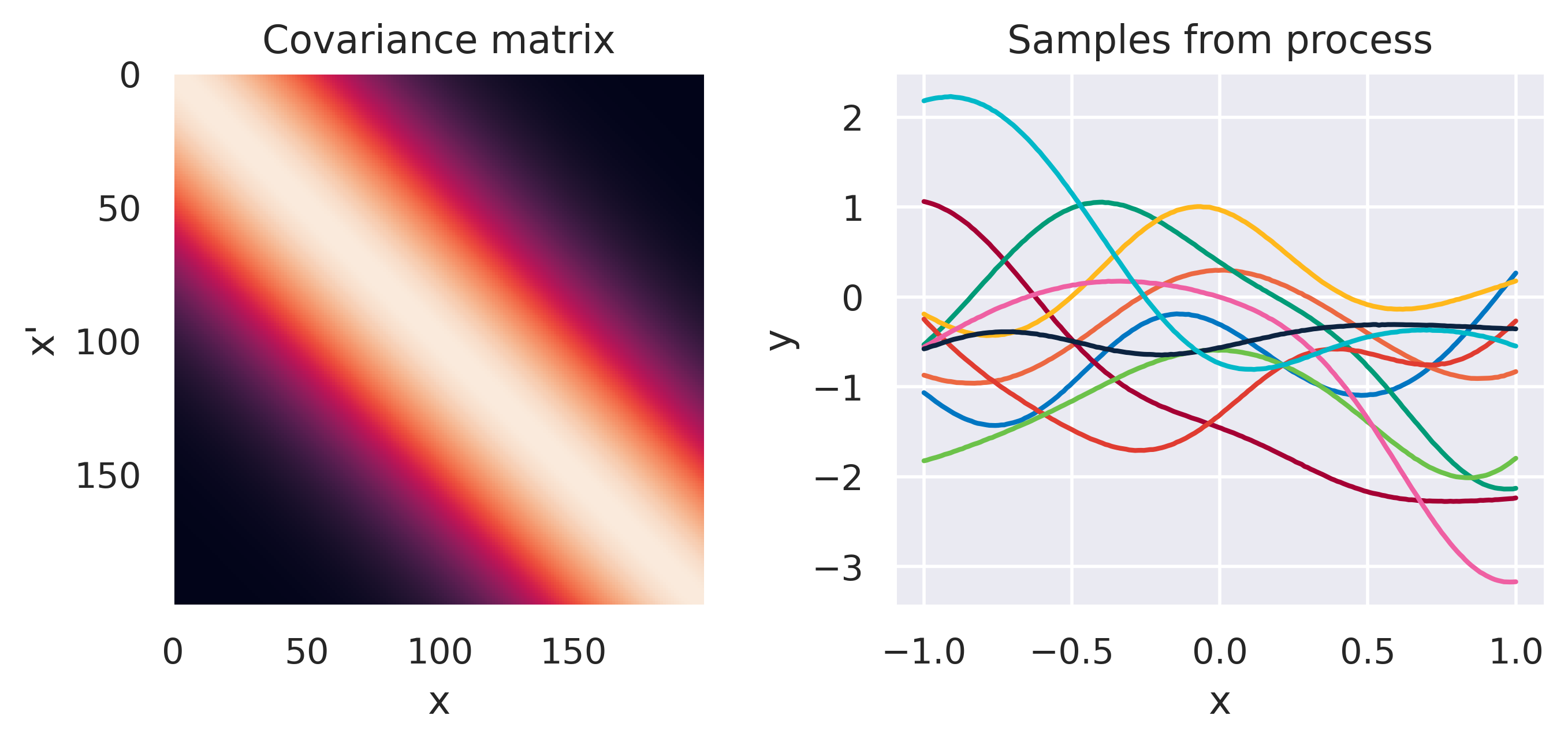
\(k(\bx,\bx') = \sigma_f^2\exp\left(\displaystyle-\frac{d^2}{2\ell^2}\right)\)
\(d = \lVert\bx-\bx'\rVert\)
\(\sigma_f=1\), \(\color{red}\ell=0.5\)
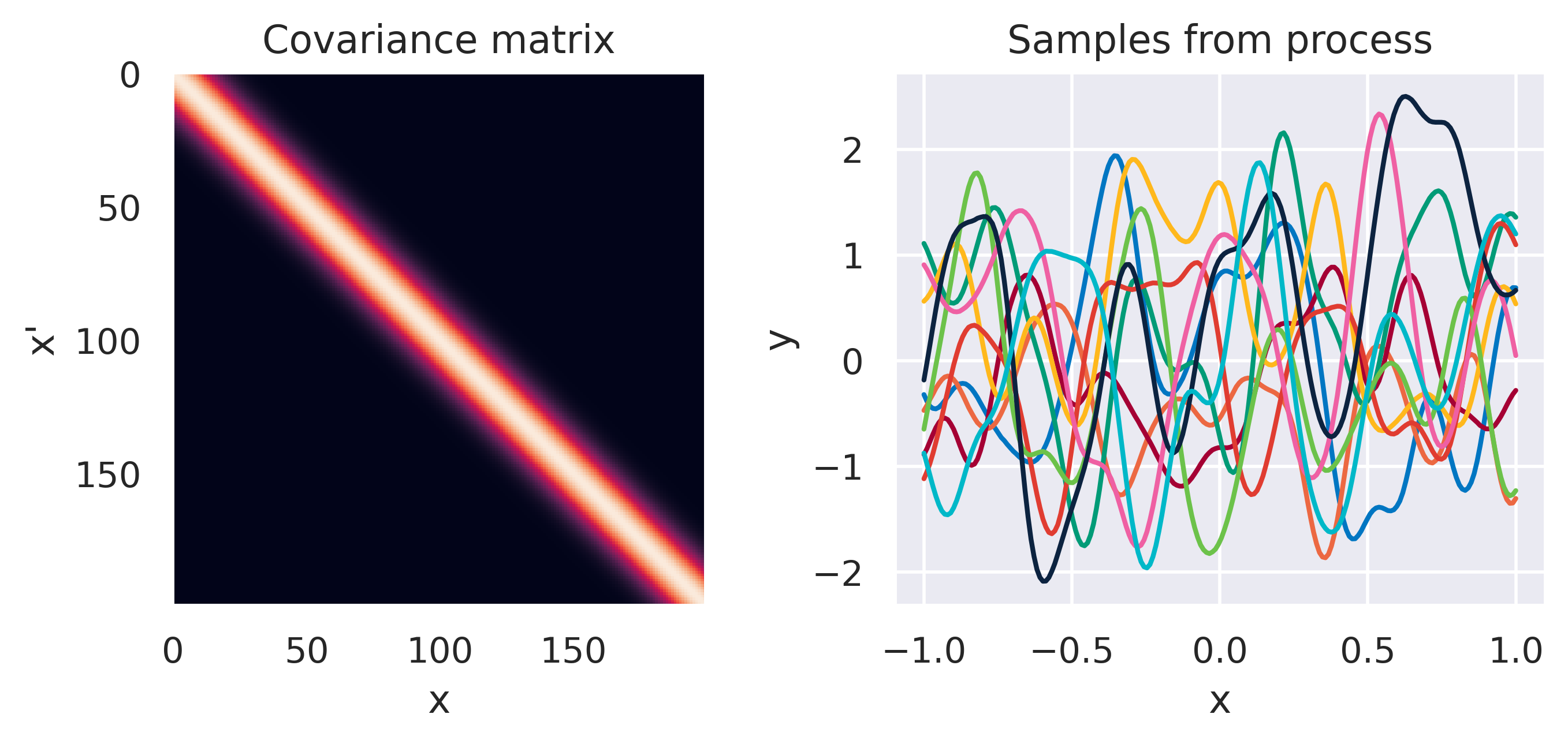
\(k(\bx,\bx') = \sigma_f^2\exp\left(\displaystyle-\frac{d^2}{2\ell^2}\right)\)
\(d = \lVert\bx-\bx'\rVert\)
\(\sigma_f=1\), \(\color{red}\ell=0.1\)
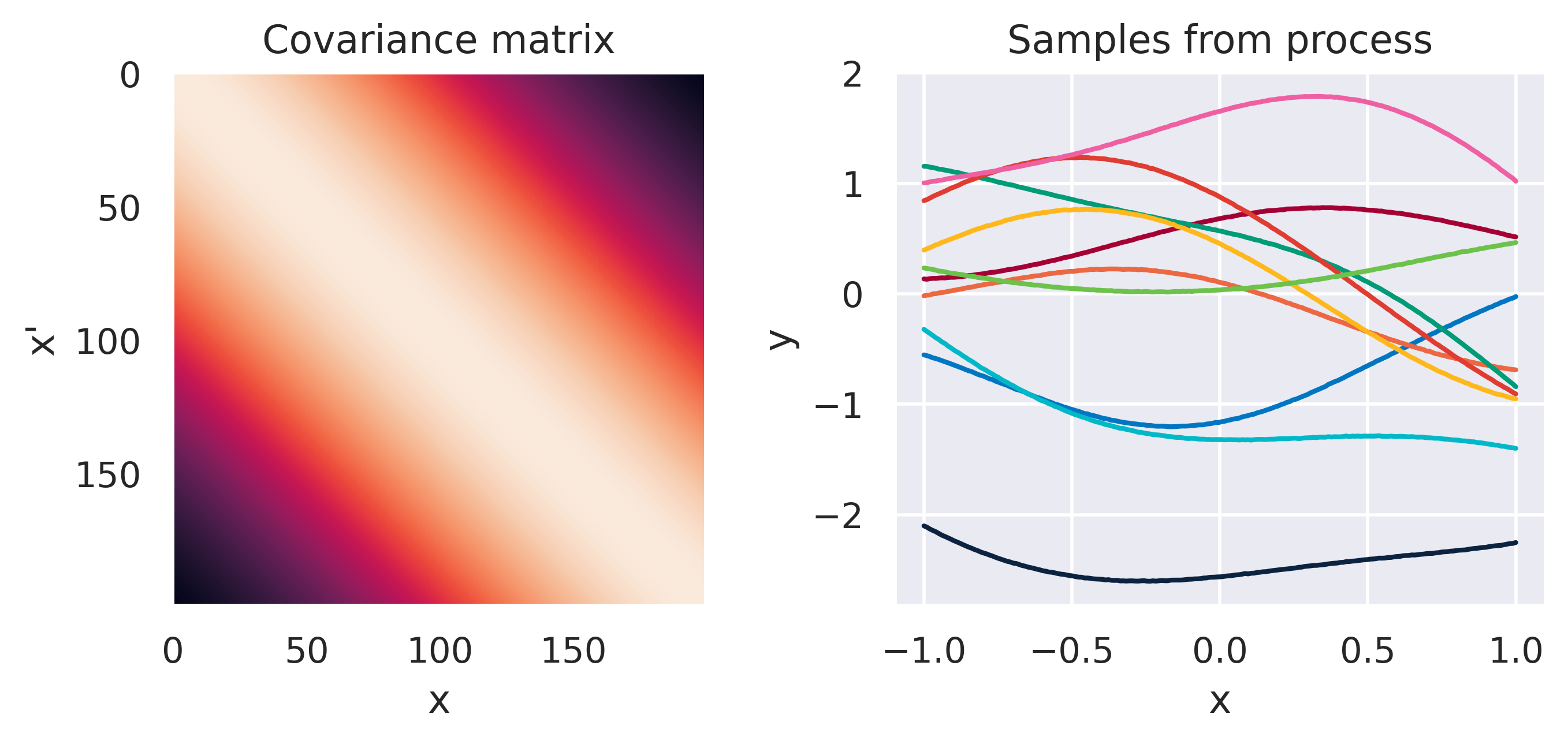
\(\tiny k(\bx,\bx') = \displaystyle\frac{\sigma_f^2}{\Gamma(\nu)2^{\nu-1}} \left( \frac{\sqrt{2\nu}d}{\ell} \right)^\nu K_\nu \left( \frac{\sqrt{2\nu}d}{\ell} \right)\)
\(d = \lVert\bx-\bx'\rVert\)
\(\color{red}\nu \rightarrow \infty\), \(\sigma_f=1\), \(\ell=1\)
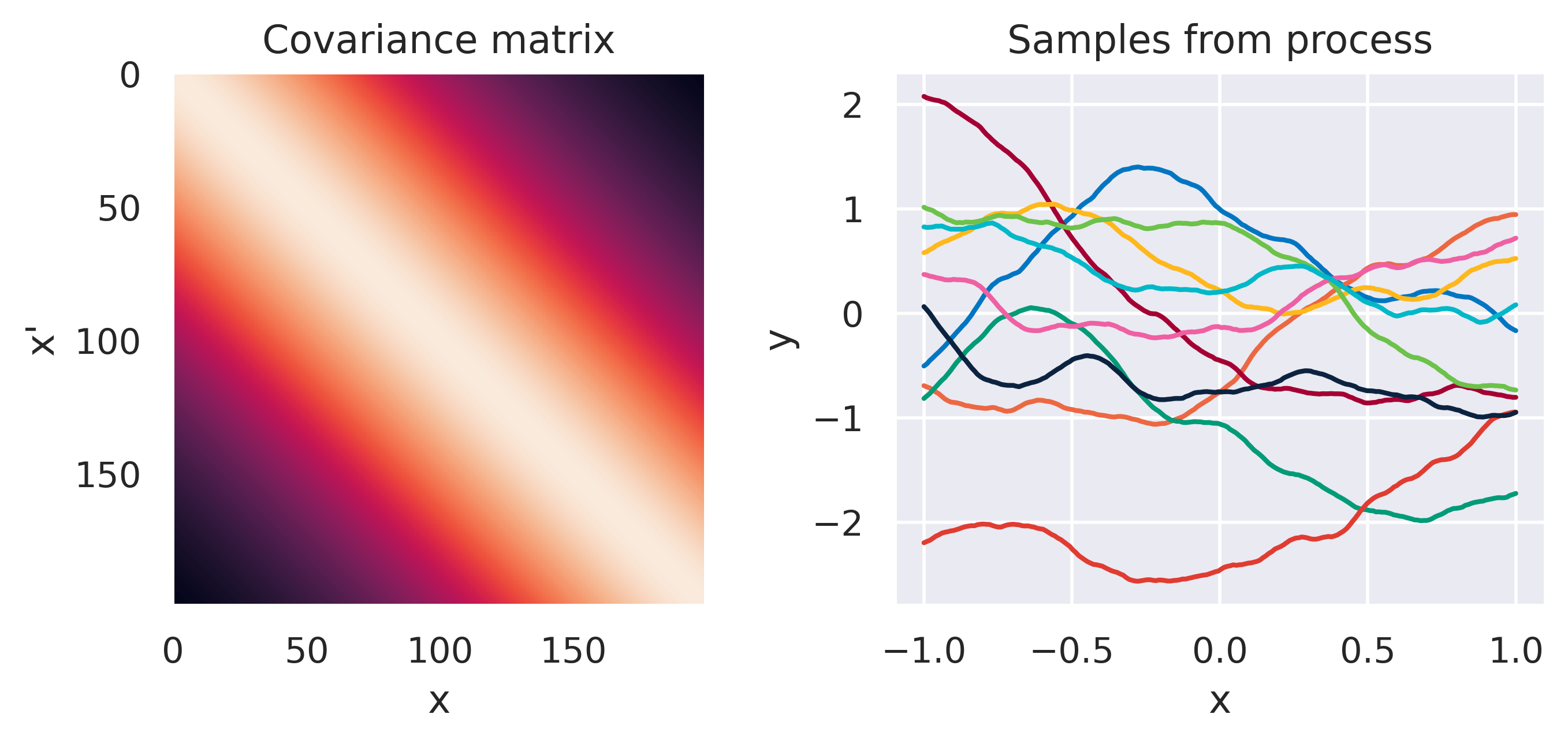
\(\tiny k(\bx,\bx') = \displaystyle\frac{\sigma_f^2}{\Gamma(\nu)2^{\nu-1}} \left( \frac{\sqrt{2\nu}d}{\ell} \right)^\nu K_\nu \left( \frac{\sqrt{2\nu}d}{\ell} \right)\)
\(d = \lVert\bx-\bx'\rVert\)
\(\color{red}\nu = 1.5\), \(\sigma_f=1\), \(\ell=1.0\)
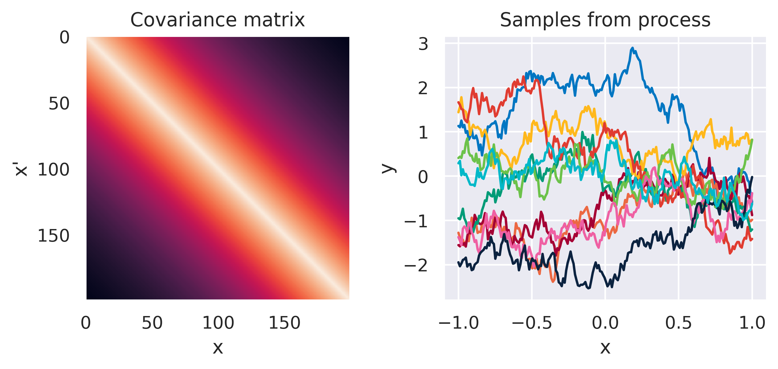
\(\tiny k(\bx,\bx') = \displaystyle\frac{\sigma_f^2}{\Gamma(\nu)2^{\nu-1}} \left( \frac{\sqrt{2\nu}d}{\ell} \right)^\nu K_\nu \left( \frac{\sqrt{2\nu}d}{\ell} \right)\)
\(d = \lVert\bx-\bx'\rVert\)
\(\color{red}\nu = 0.5\), \(\sigma_f=1\), \(\ell=1.0\)
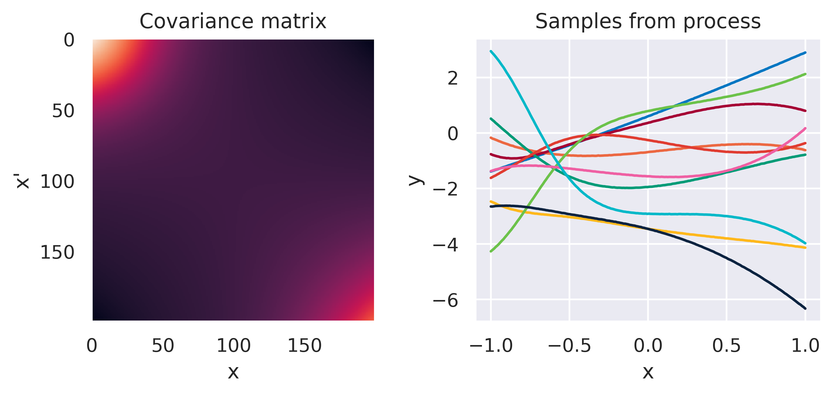
\(\small k(\bx,\bx') = 2k_1(\bx,\bx') + k_2(\bx,\bx')\)
\(\small k_1(\bx,\bx') = k_\mathrm{RBF}(M=1,s=0.3)\)
\(\small k_2(\bx,\bx') = k_\mathrm{Poly}(M=3)\)
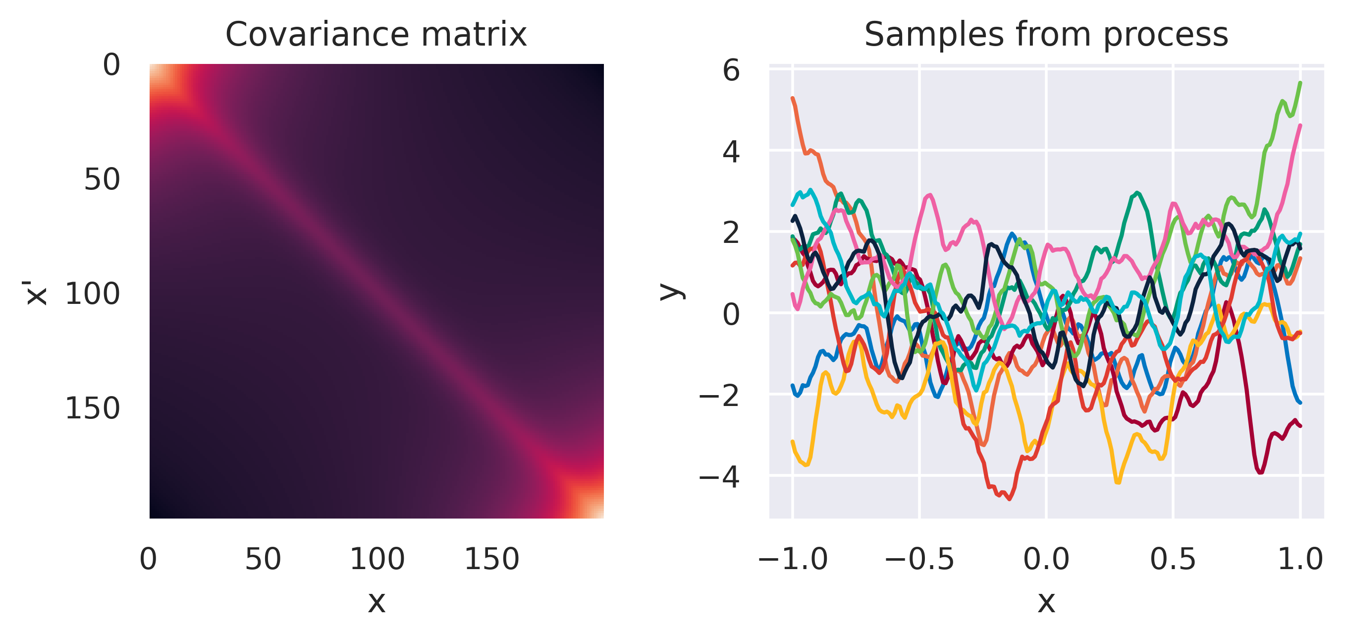
\(\small k(\bx,\bx') = k_1(\bx,\bx') + k_2(\bx,\bx')\)
\(\small k_1(\bx,\bx') = k_\mathrm{Matern}(\ell=0.1)\)
\(\small k_2(\bx,\bx') = k_\mathrm{Poly}(M=5)\)
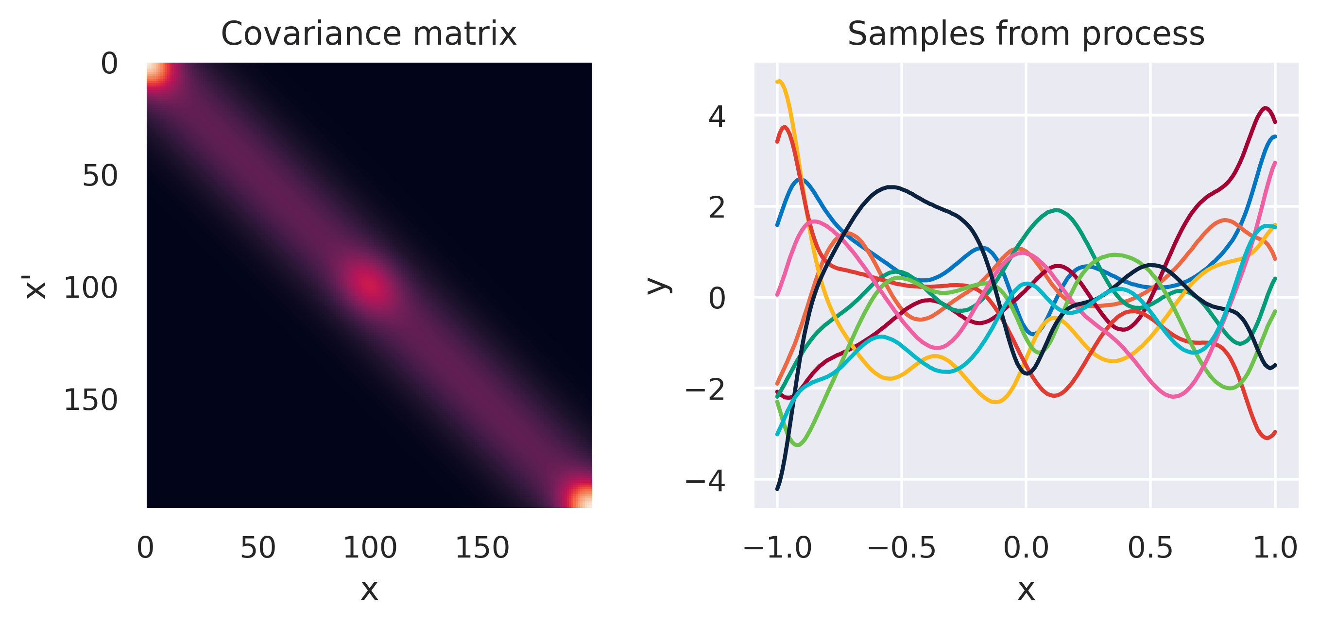
\(\small k(\bx,\bx') = k_1\cdot k_2\cdot k_3\)
\(\small k_1(\bx,\bx') = k_\mathrm{SE}(\ell=0.2)\)
\(\small k_2(\bx,\bx') = k_\mathrm{RBF}(M=3,s=0.1)\)
\(\small k_3(\bx,\bx') = k_\mathrm{RBF}(M=2,s=0.1)\)
Note how different kernels lead to different covariance structures, which in turn change how the functions drawn from the process behave. Also interesting is to note how adding more radial basis functions makes \(\mbf{K}\) look more and more like the one we get with the squared exponential kernel. This is not a coincidence, and illustrates the main advantage of the kernel approach: a function \(y(\bx)\) described by a squared exponential kernel is equivalent to a radial basis function model with an infinite number of bases. In weight space this would mean the vector \(\bw\) would have infinite entries, making the model intractable. But in function space this powerful model with essentially infinite flexibility model becomes usable.
Further Reading
How else can we build valid kernels? Apart from the operations you see for the hybrid kernels above, there are many other ways. You can read pages 295 and 296 to find out, if you are curious.
bishop-prml
