Empirical Bayes

To wrap up our discussion on GPs, we talk about model selection. Recall that we must pick a kernel for our Gaussian Process, for instance the Squared Exponential:

(83)\[ k(\bx,\bx') = \sigma_f^2\exp\left(\displaystyle-\frac{1}{2\ell^2}\lVert\bx-\bx'\rVert^2\right) \]

Given that our choice of kernel is fixed, the model selection problem becomes one of determining suitable values for hyperparameters \(\sigma_f\), \(\ell\) and the noise \(\beta\).

In Learning and Model Selection, we did the same for weight-space models by marginalizing \(\bw\) to obtain an expression for \(p(\mbf{t})\), the marginal likelihood, or evidence function. We then used Empirical Bayes to compute \(\alpha\) and \(\beta\) that maximized this evidence.

For GPs the operation is exactly the same, but getting to the evidence is much easier now. Recall from Eq. (79) that we already have an expression for \(p(\mbf{t})\):

(84)\[ p(\mbf{t}) = \gauss\left( \mbf{t}\left\vert\right.\mbf{0}, K\left(\mbf{X},\mbf{X}\right) + \beta^{-1}\mbf{I} \right) \]

Since this is nothing more than a multivariate Gaussian, we can easily compute the log likelihood of our training dataset:

(85)\[ \ln p(\mbf{t}\vert\sigma_f,\ell,\beta) = \displaystyle -\frac{1}{2}\ln\vert\mbf{K}+\beta^{-1}\mbf{I}\vert -\frac{1}{2}\mbf{t}^\T\left(\mbf{K}+\beta^{-1}\mbf{I}\right)^{-1}\mbf{t} -\frac{N}{2}\ln\left(2\pi\right) \]

where \(N\) is the size of our dataset and the dependencies on \(\sigma_f\) and \(\ell\) come from \(\mbf{K}\). We can then use an optimizer to maximize this expression.

Click through the tabs below to observe the optimization progress of the regression example with \(N=5\) data points we have shown before. The figure captions show the hyperparameter and log marginal likelihood values as more optimizer iterations are run. Note how the likelihood gradually increases, starting from a severely underfit model, passsing through a somewhat overfit model and ending at a well-balanced model. Crucially, we do this without having to define a validation dataset, and therefore using all of our data to make predictions.

Initial guess

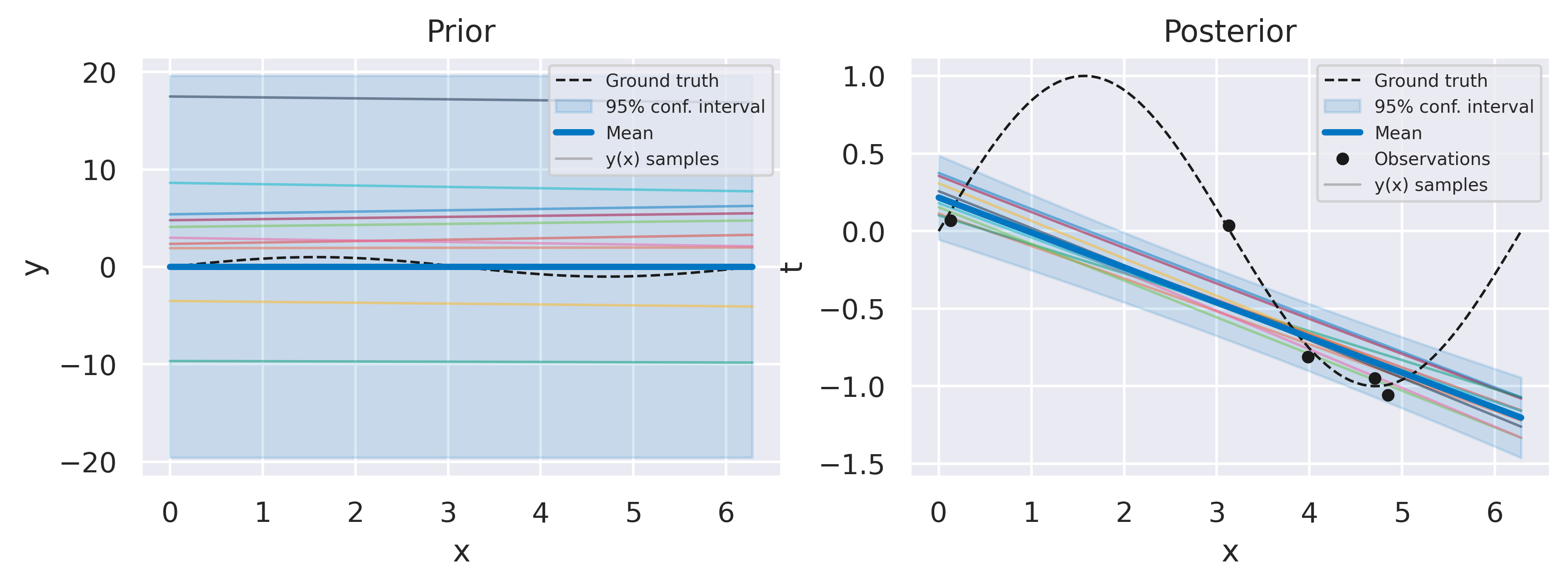
Fig. 32 Prior and posterior distributions, with \(\sigma_f=100\), \(\ell=100\), \(\beta=100\), \(\ln p(\mbf{t}) = -19.91\)

25% optimized

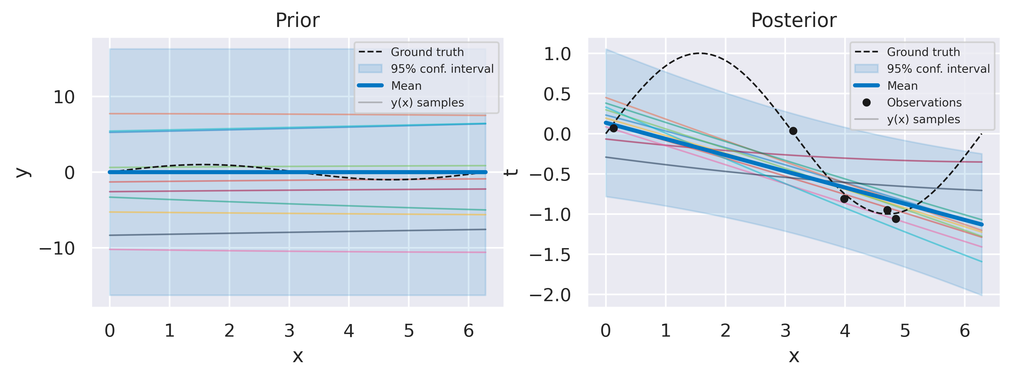
Fig. 33 Prior and posterior distributions, with \(\sigma_f=68.9\), \(\ell=40.8\), \(\beta=8.3\), \(\ln p(\mbf{t}) = -6.21\)

50% optimized

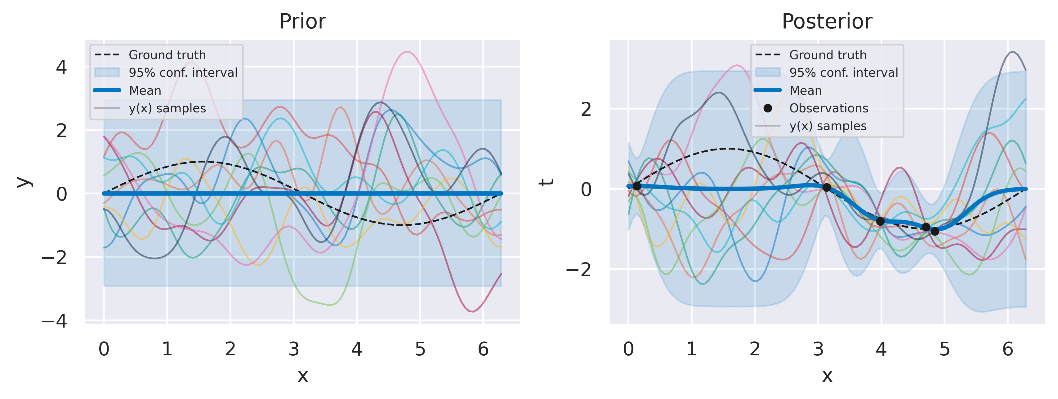
Fig. 34 Prior and posterior distributions, with \(\sigma_f=2.1\), \(\ell=0.4282\), \(\beta=16.1\), \(\ln p(\mbf{t}) = -5.98\)

75% optimized

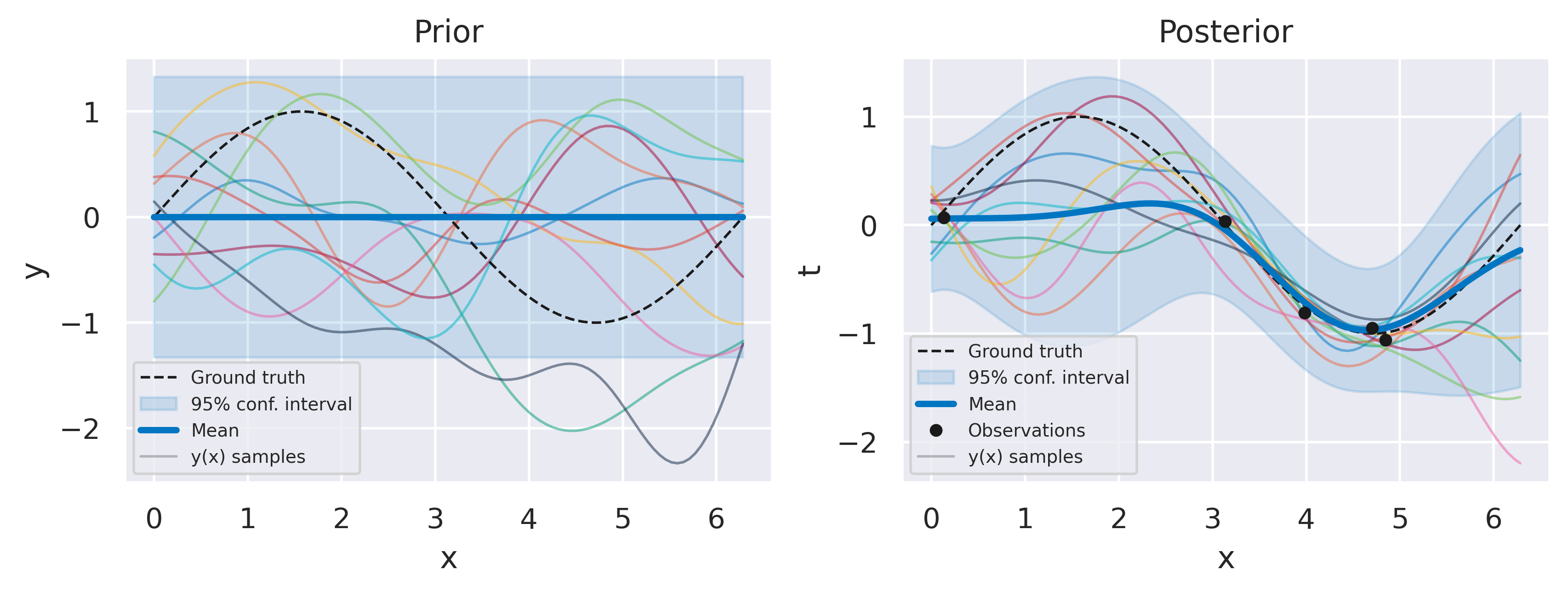
Fig. 35 Prior and posterior distributions, with \(\sigma_f=0.4\), \(\ell=0.9\), \(\beta=16.7575\), \(\ln p(\mbf{t}) = -2.98\)

Final values

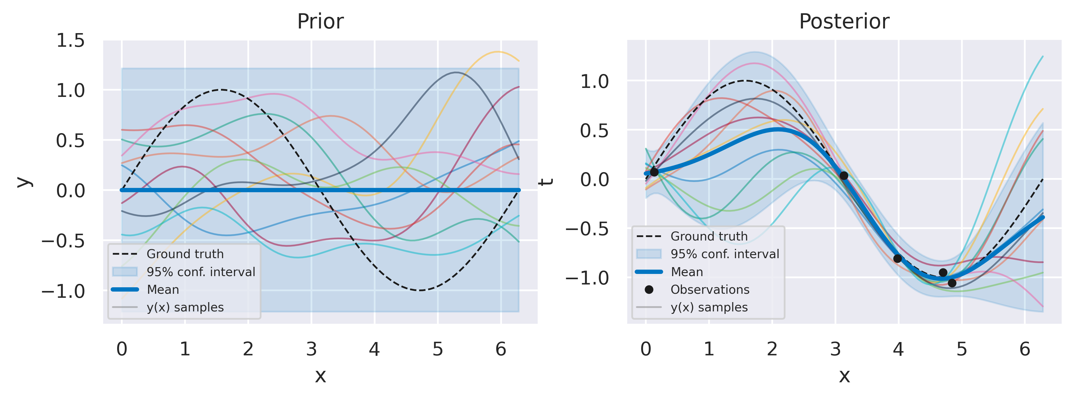
Fig. 36 Prior and posterior distributions, with \(\sigma_f=0.4\), \(\ell=1.2\), \(\beta=167.1\), \(\ln p(\mbf{t}) = -2.25\)