Active Learning

The Bayesian approach of weighing prior beliefs and observations lends itself well to situations in which a complete dataset is not available from the start but data is instead coming in gradually in a sequential manner:

Batch learning

A dataset \(\mathcal{D}\) with several observations is already available before training. Bayes’ Theorem is used to go directly from the no-data initial prior to the final posterior distribution.

Active learning

We start with an empty dataset and only the initial prior distribution. A posterior is computed when new data comes in and this posterior becomes the prior for the next update. This is repeated until all the data has been observed.

Here we demonstrate this approach with a couple of examples. As before we start from a prior over our parameters:

(51)\[ p(\mathbf{w}) = \mathcal{N}\left(\mathbf{w}\vert\boldsymbol{0},\alpha^{-1}\mathbf{I}\right) \]

Using the same conditioning approach as before, we get for the first data point:

(52)\[ p(\mathbf{w}\vert\mathbf{t}) = \mathcal{N}\left(\mathbf{w}\vert\mathbf{m}_1,\mathbf{S}_1\right) \]

(53)\[ \mathbf{m}_1 = \beta\mathbf{S}_1\boldsymbol{\phi}(\mathbf{x}_1)^\mathrm{T}t_1 \]

(54)\[ \mathbf{S}_1^{-1} = \alpha\mathbf{I} + \beta\boldsymbol{\phi}(\mathbf{x}_1)^\mathrm{T}\boldsymbol{\phi}(\mathbf{x}_1) \]

Note that we now only compute the basis functions for a single input vector \(\mathbf{x}_1\) and condition on only a single target \(t_1\) (it was a vector in Eq. (45)).

To observe a second data point we just use Eq. (52) as our new prior and repeat the process. Using the standard expressions from before we get:

(55)\[ p(\mathbf{w}\vert\mathbf{t}) = \mathcal{N}\left(\mathbf{w}\vert\mathbf{m}_2,\mathbf{S}_2\right) \]

(56)\[ \mathbf{m}_2 = \mathbf{S}_2\left(\mathbf{S}_1^{-1}\mathbf{m}_1 + \beta\boldsymbol{\phi}(\mathbf{x}_2)^\mathrm{T}t_2\right) \]

(57)\[ \mathbf{S}_2^{-1} = \mathbf{S}_1^{-1} + \beta\boldsymbol{\phi}(\mathbf{x}_2)^\mathrm{T}\boldsymbol{\phi}(\mathbf{x}_2) \]

and recalling that \(\mathbf{m}_0=\boldsymbol{0}\) in Eq. (51), we see that we have exactly the same expressions for the second update but with the first posterior acting as the new prior.

The above can be generalized as:

(58)\[ p(\mathbf{w}\vert\mathbf{t}) = \mathcal{N}\left(\mathbf{w}\vert\mathbf{m}_\mathrm{new},\mathbf{S}_\mathrm{new}\right) \]

(59)\[ \mathbf{m}_\mathrm{new} = \mathbf{S}_\mathrm{new}\left(\mathbf{S}_\mathrm{old}^{-1}\mathbf{m}_\mathrm{old} + \beta\boldsymbol{\phi}(\mathbf{x}_\mathrm{new})^\mathrm{T}t_\mathrm{new}\right) \]

(60)\[ \mathbf{S}_\mathrm{new}^{-1} = \mathbf{S}_\mathrm{old}^{-1} + \beta\boldsymbol{\phi}(\mathbf{x}_\mathrm{new})^\mathrm{T}\boldsymbol{\phi}(\mathbf{x}_\mathrm{new}) \]

and observing one point at a time is not strictly necessary, we could also observe data in chunks and the same expressions would hold as long as we arrange \(\mathbf{t}\) and \(\boldsymbol{\Phi}\) in their proper vector/matrix forms.

Click through the tabs below to see an example of this procedure. We start with a prior model with Radial Basis Functions and observe one data point at a time. On the left plots you can see 10 sets of weights sampled from our prior/posterior distribution and the corresponding predictions they give. This is a nice feature of the Bayesian approach: we do not end up with a single trained model but with a bag of models we can draw from.

Prior

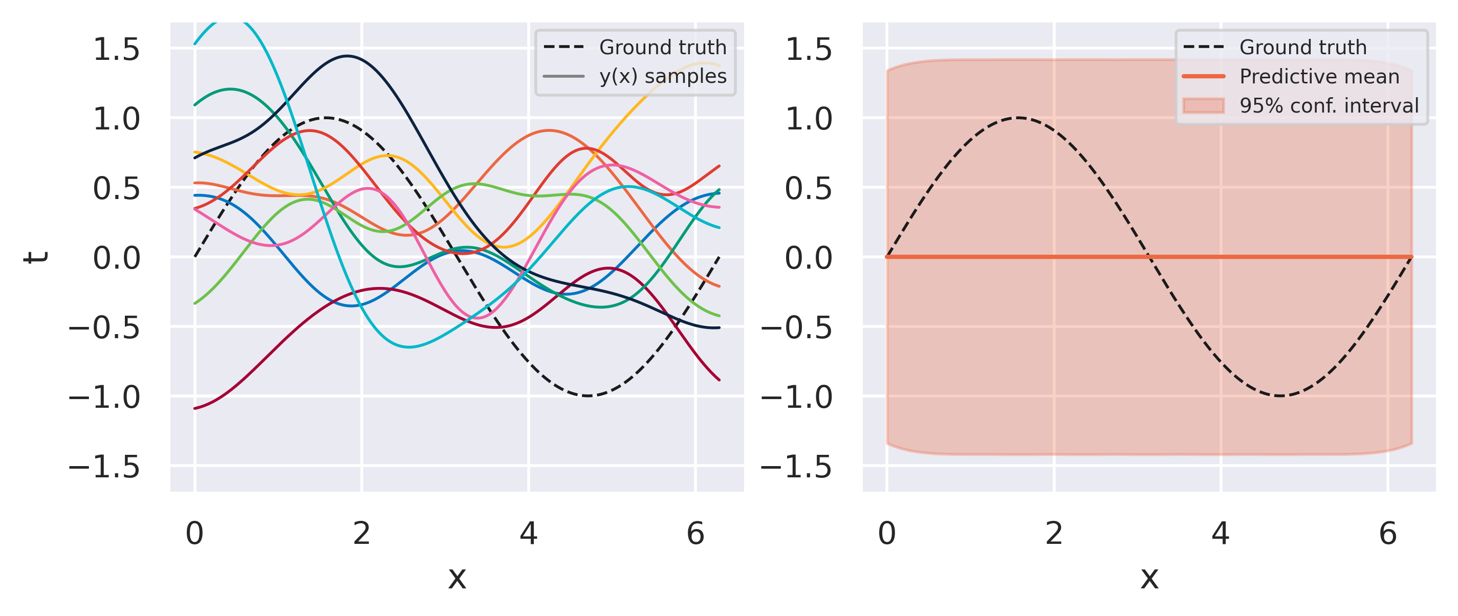
Fig. 14 Model behavior under only our prior assumptions

1 data point

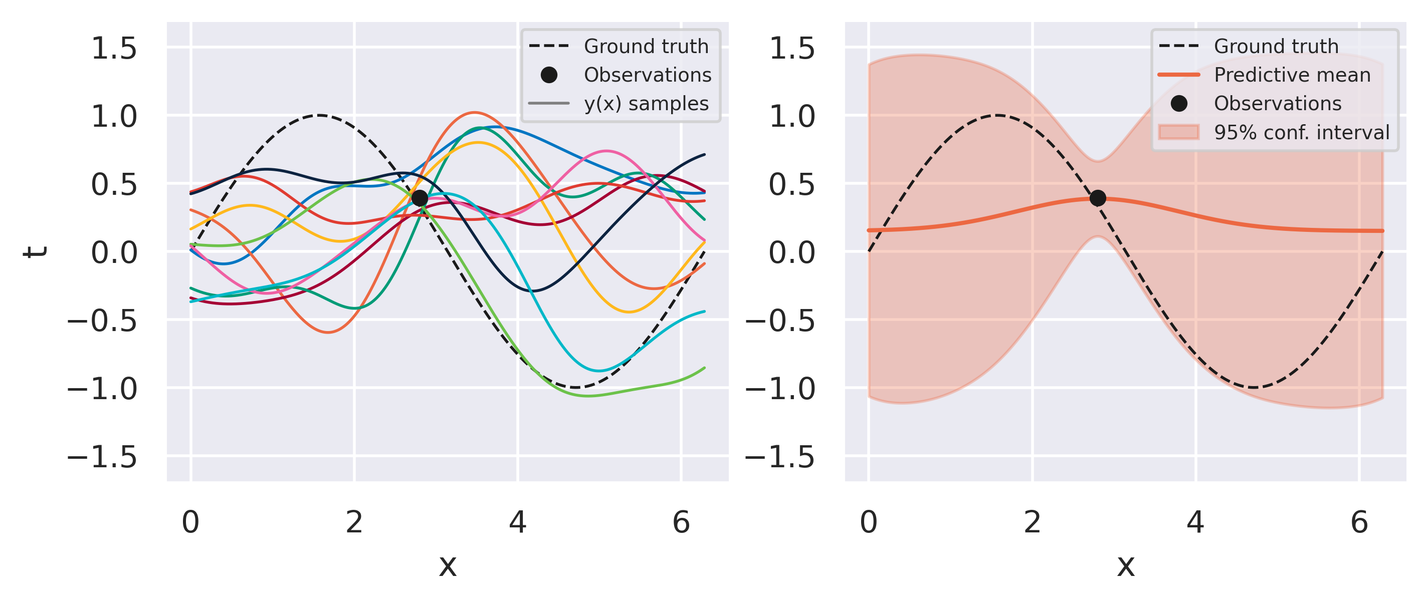
Fig. 15 Bayesian fit with one observation

2 data points

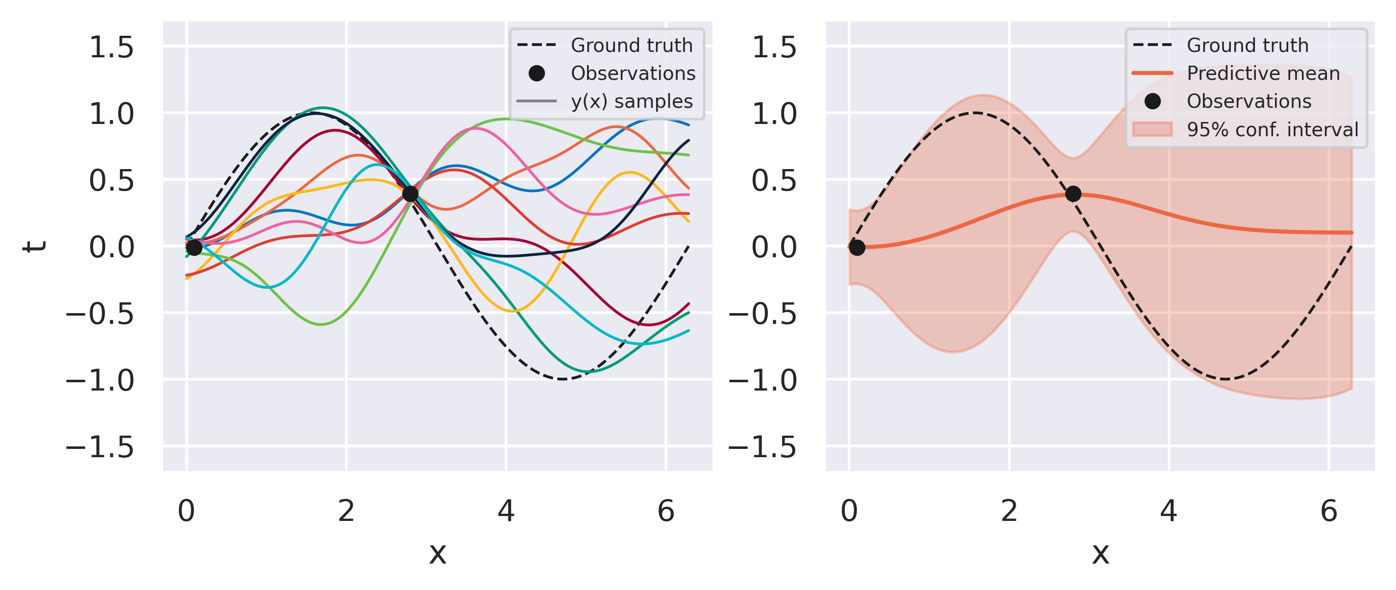
Fig. 16 Bayesian fit with two observations

3 data points

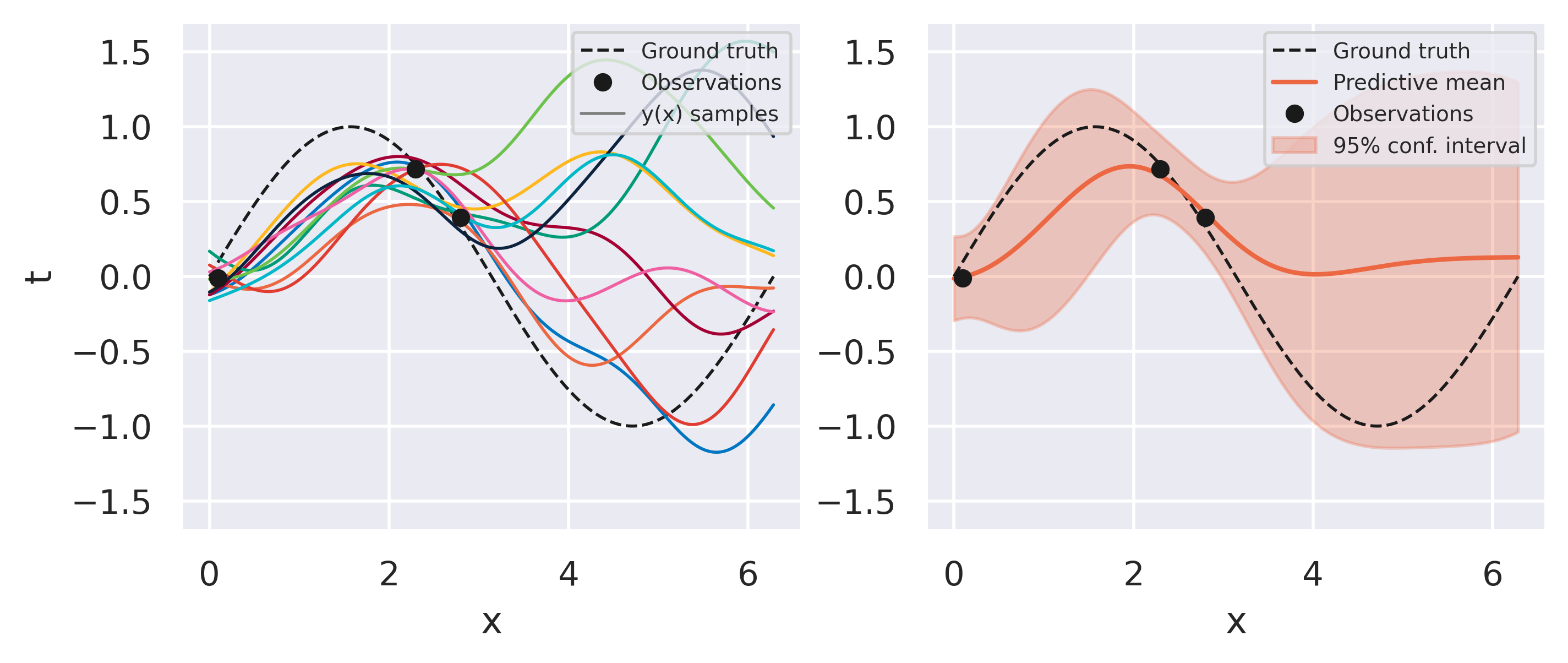
Fig. 17 Bayesian fit with three observations

4 data points

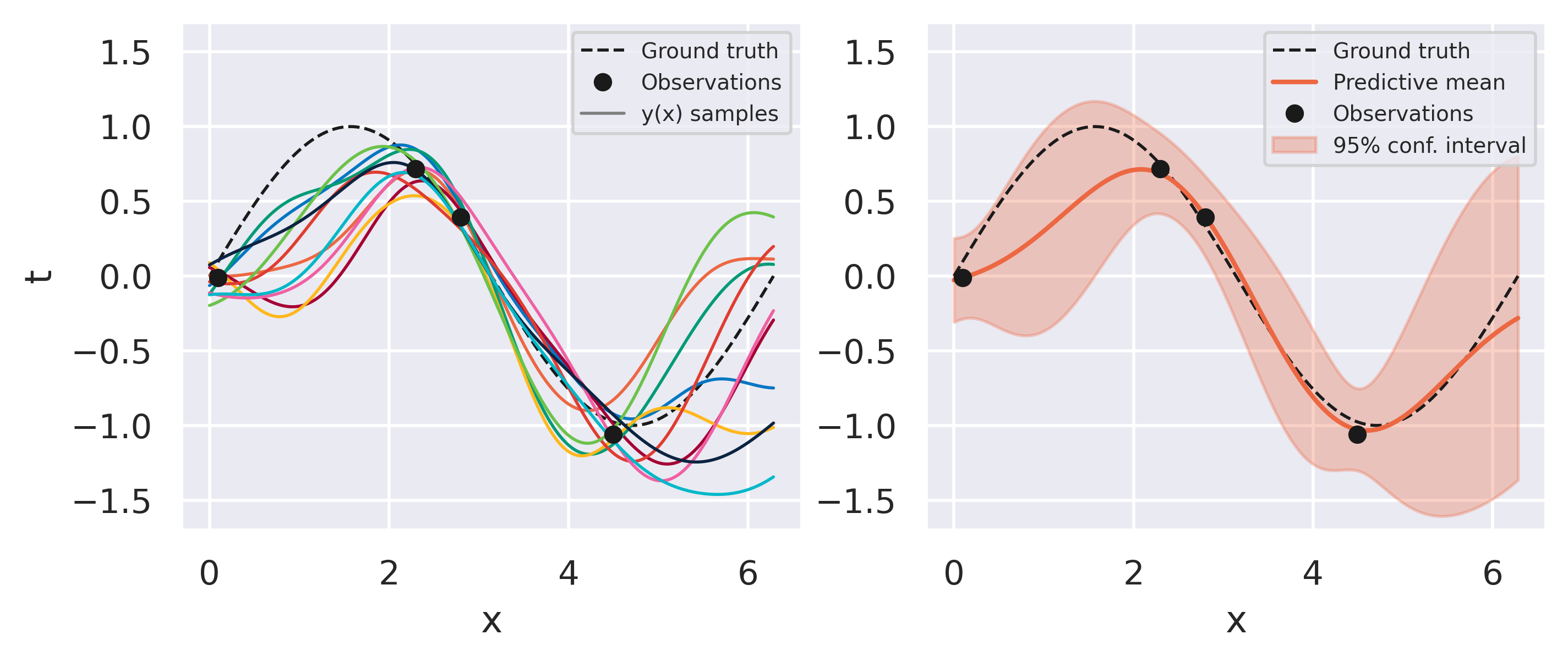
Fig. 18 Bayesian fit with four observations

5 data points

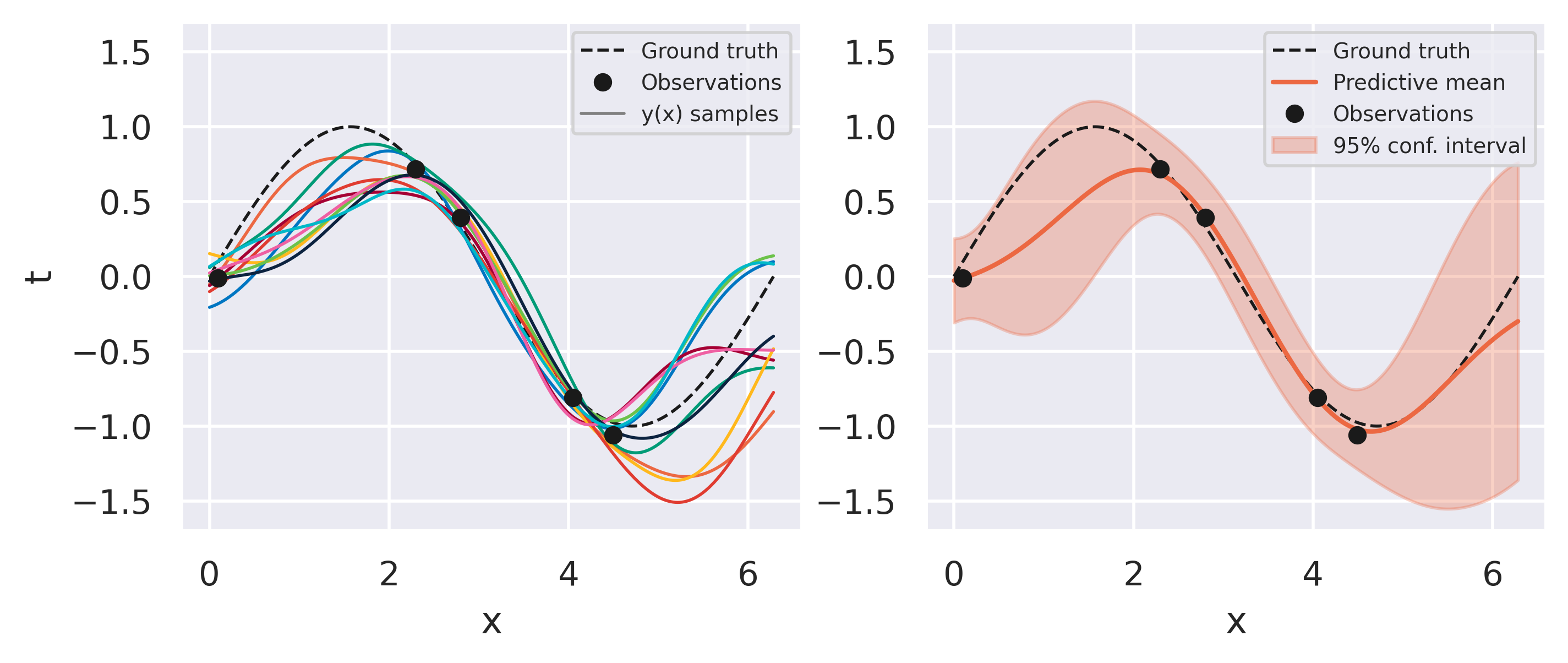
Fig. 19 Bayesian fit with five observations

What can you observe from the results above? Note how models sampled from the initial prior are quite uninformed. As soon as some data is observed, the posterior space of possible models becomes more and more constrained to agree with the observed points. Note also that instead of drawing models from our posterior we can conveniently just look at the predictive mean and variance on the right-hand plots. This already conveys enough information since our all our distributions are Gaussian.

A deeper look

The figures above show what happens with our final model as we observe data. They however only give an indirect idea of how \(p(\mathbf{w}\vert\mathbf{t}\)) is changing as more data is added. Since the functions above are of the form \(y = \mathbf{w}^\mathrm{T}\boldsymbol{\phi}(\mathbf{x})\) with 10 weights, it is difficult to visualize their joint probability distribution in 10 dimensions.

To make that visible, the figures below show a simple linear model with a single weight (the intercept is fixed at zero):

(61)\[ p(t\vert w,\beta) = \mathcal{N}(t\vert wx,\beta^{-1}) \quad\quad p(w\vert\alpha) = \mathcal{N}(w\vert 0,\alpha^{-1}) \]

which in this case means \(\boldsymbol{\phi}(\mathbf{x})=[x]\). Again we start with no observations and fix \(\alpha=100\) and \(\beta=40\). Click through the tabs below to see how training evolves as more data becomes available:

Prior

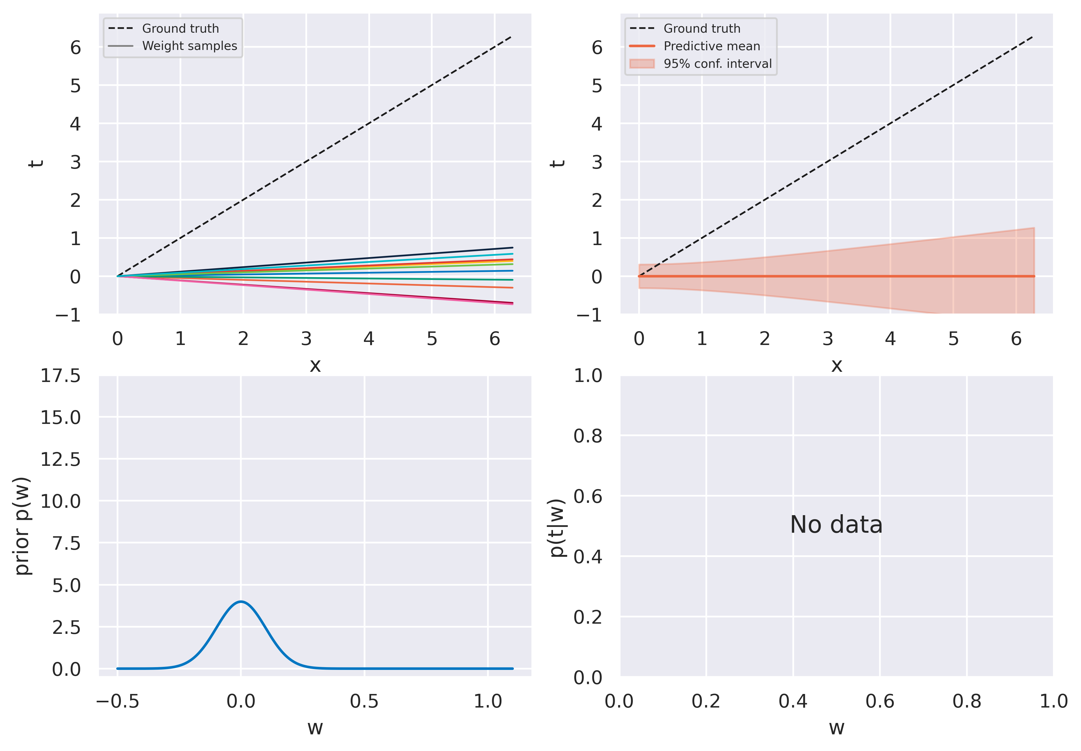
Fig. 20 Model behavior under only our prior assumptions

1 data point

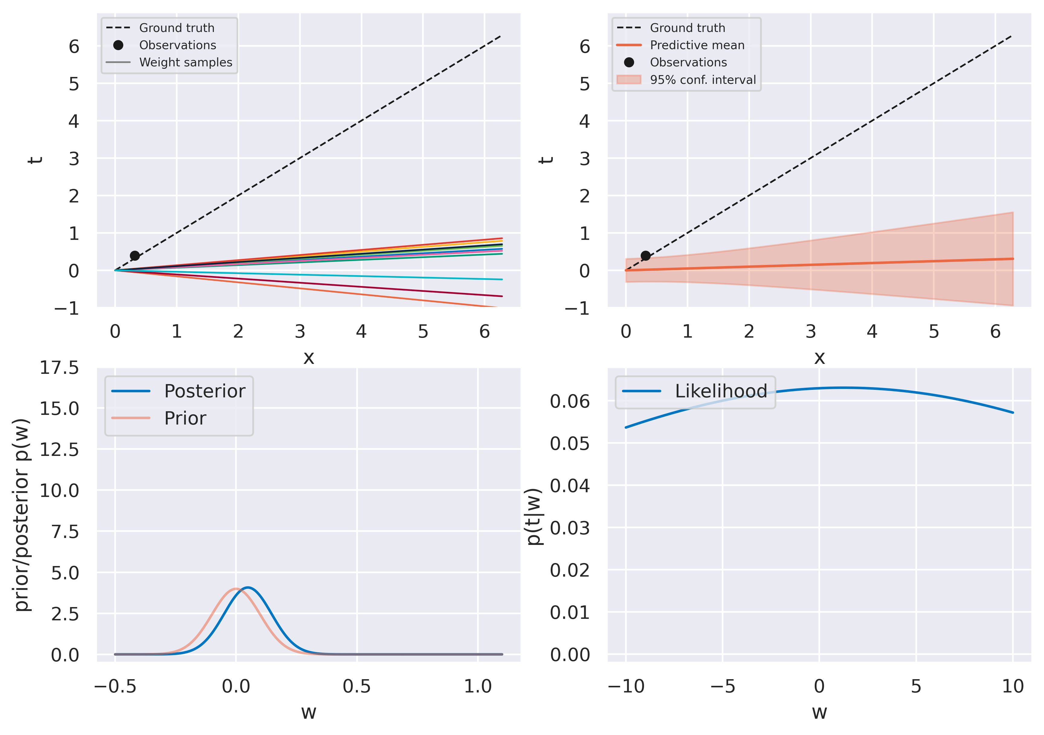
Fig. 21 Bayesian fit with one observation

2 data points

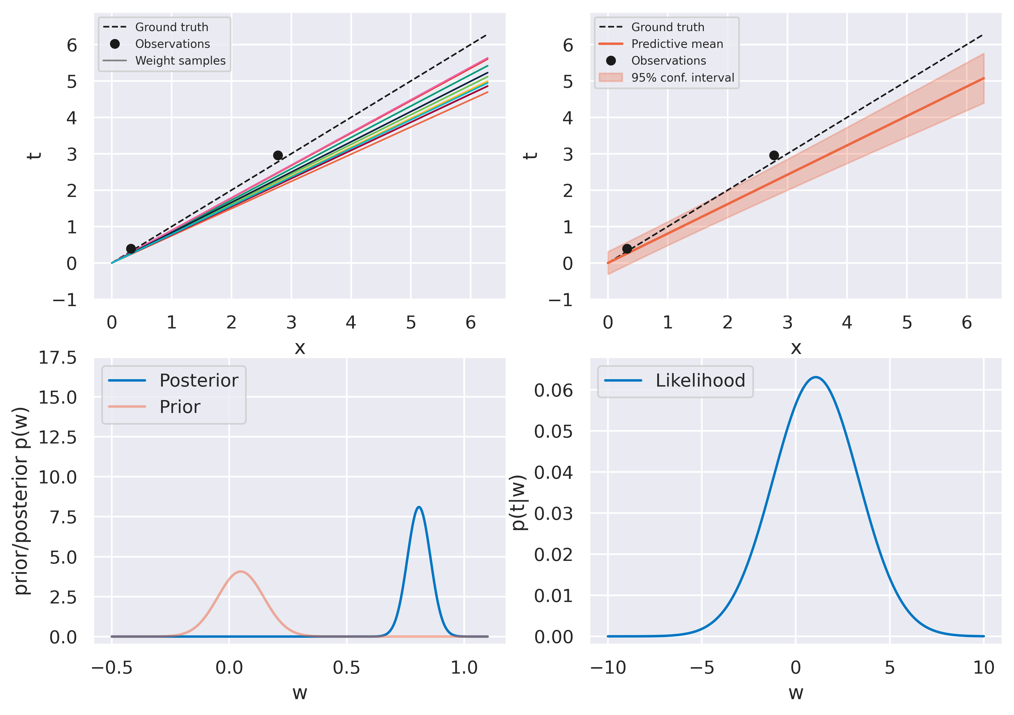
Fig. 22 Bayesian fit with two observations

3 data points

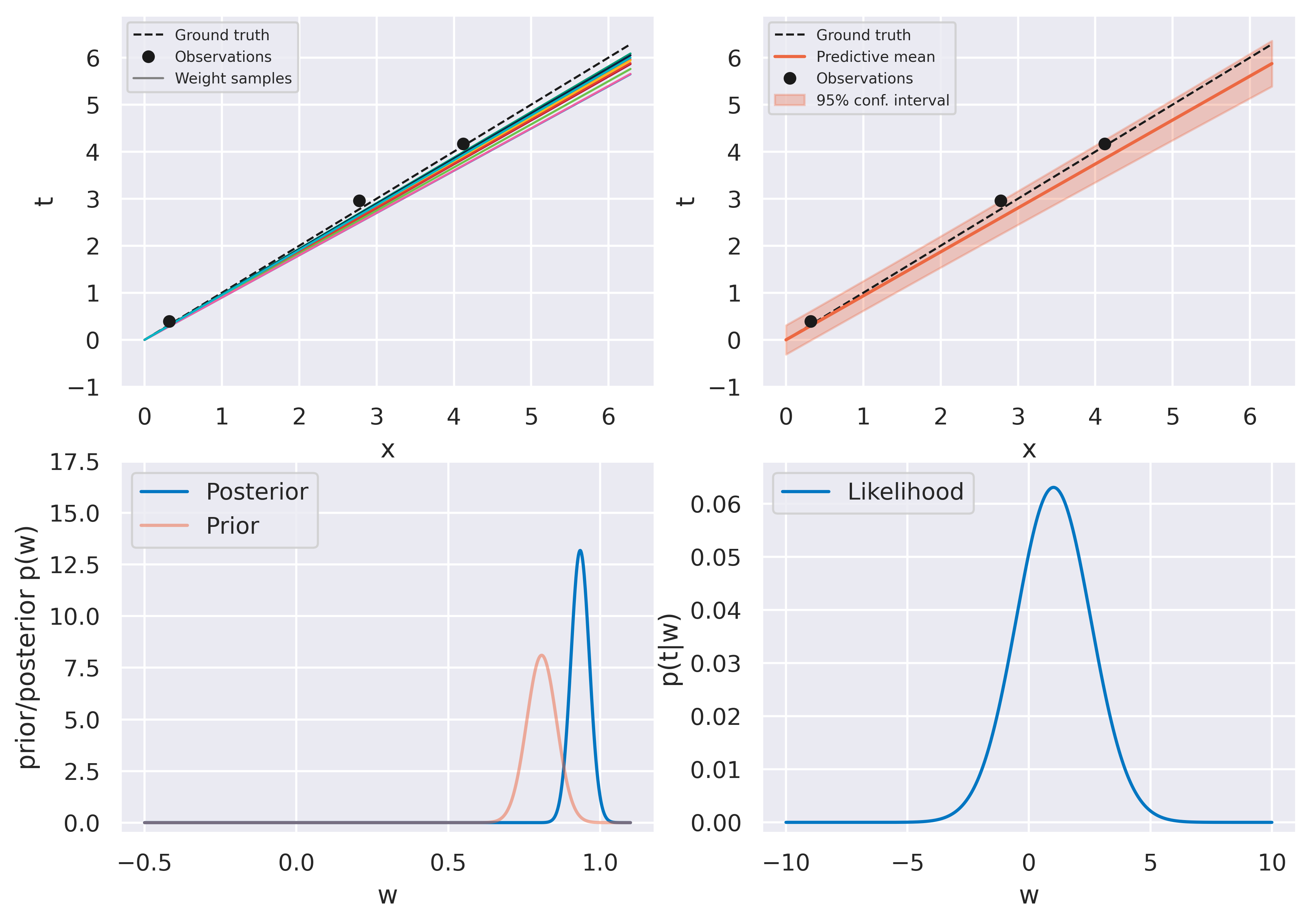
Fig. 23 Bayesian fit with three observations

4 data points

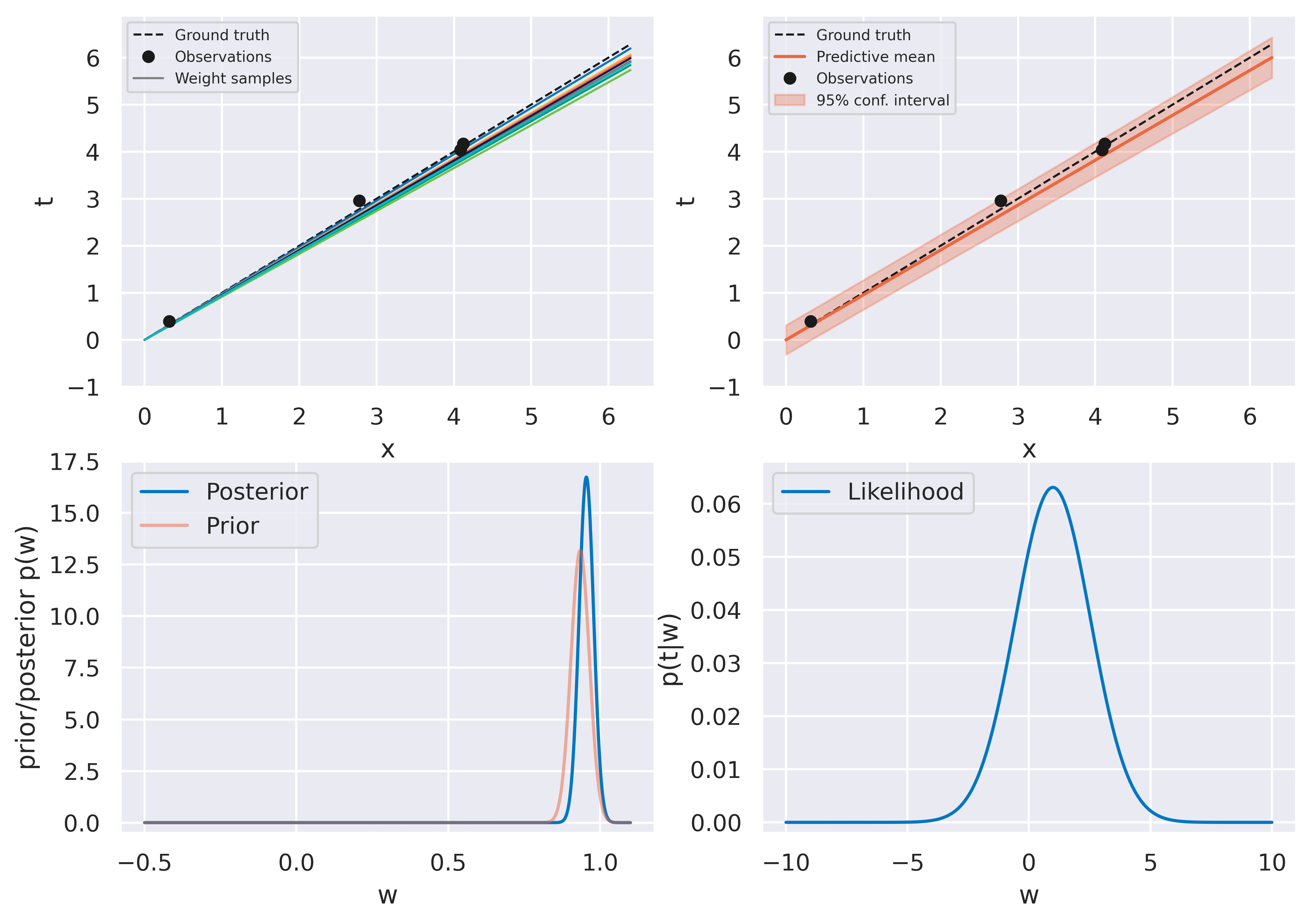
Fig. 24 Bayesian fit with four observations

5 data points

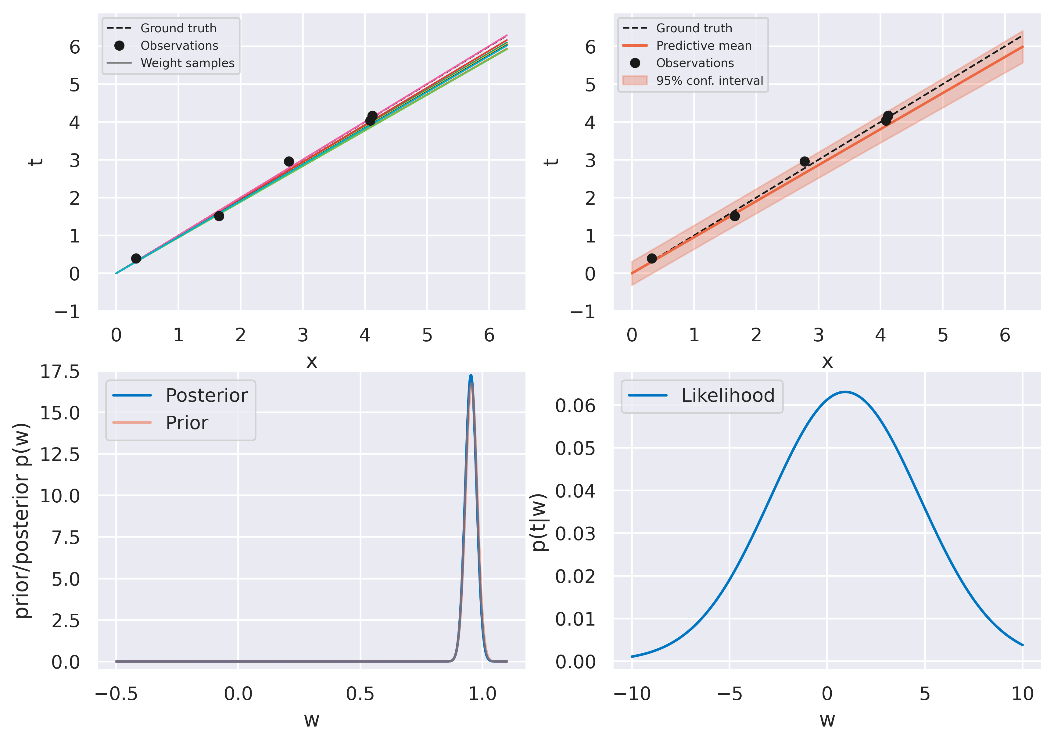
Fig. 25 Bayesian fit with five observations

The figures on the top row should look familiar. We again start with an uninformed bag of models and they evolve to a more constrained version as more data is observed. The bottom row shows some new insights. On the left we see the actual probability distribution \(p(w)\), either prior or posterior.

On the right we see a plot of the likelihood function \(p(t\vert w)\). Recall this is a distribution on \(t\), and therefore not on \(w\)! When plotting it against \(w\) (on which it does depend), we call it likelihood function instead of probability distribution to make the distinction clear. The likelihood function provides a measure of how likely different values of \(w\) would make the observation of the data point currently being assimilated. It therefore provides a push towards certain values of \(w\) which is weighed against the current prior \(p(w)\).

Note how observing the first point has little effect on the posterior: it is so close to the origin that the likelihood function becomes quite spread and moves the posterior very little. We can read this as “our current observation might just as well be explained with our observation noise \(\beta\) regardless of what \(w\) is”. Observing subsequent points gradually moves the posterior towards the ground truth value \(w_\mathrm{true}=1\) and the distribution becomes more highly peaked, as we would expect.

At the limit of infinite observations:

(62)\[ N\to\infty\quad\Rightarrow\quad m_\infty\to w_\mathrm{MLE},\quad S_\infty\to 0 \]

This is a very satisfying result: when evidence is absolutely overwhelming, our prior beliefs should be completely discarded and we should just rely purely on what the data says.

Further Reading

You can now finish reading Section 3.3.1. Figure 3.7 contains a two-dimensional version of the example above which you can relate to what you have seen here.

bishop-prml