Linear Basis Function Models#
Here we come back to basis function models for regression but now through a Bayesian perspective. To make the discussion easier to follow, we again start at decision theory. We also draw parallels with the frequentist treatment we have seen before.
Decision theory and observation model#
We again have a process \(p(\mathbf{x},t)\) we would like to model with a regression function \(y(\mathbf{x})\). In doing that we incur a loss \(L\) whose expectation is:
And we have seen in Decision Theory that the best option for \(y(\mathbf{x})\) is:
We must therefore come up with an expression for \(p(t\vert\mathbf{x})\). To make our lives easier, we opt to model this with a Gaussian. It is an attractive choice because its expectation is simply its mean.
This leads to the observation model:
with \(\beta^{-1}\) being a variance parameter. Next we specify the shape of \(y(\mathbf{x})\).
Further Reading
For an extended discussion on decision theory for regression, read the short Section 1.5.5.
bishop-prml
Graph model and joint distribution#
To give \(y(\mathbf{x})\) some shape, we again go for a set of basis functions \(\boldsymbol{\phi}(\mathbf{x})\) which we assume are known and fixed. To make the model trainable we assume these basis functions are scaled by a set of weights \(\mathbf{w}\):
We can pick different basis functions for different applications. Click below for a few examples:
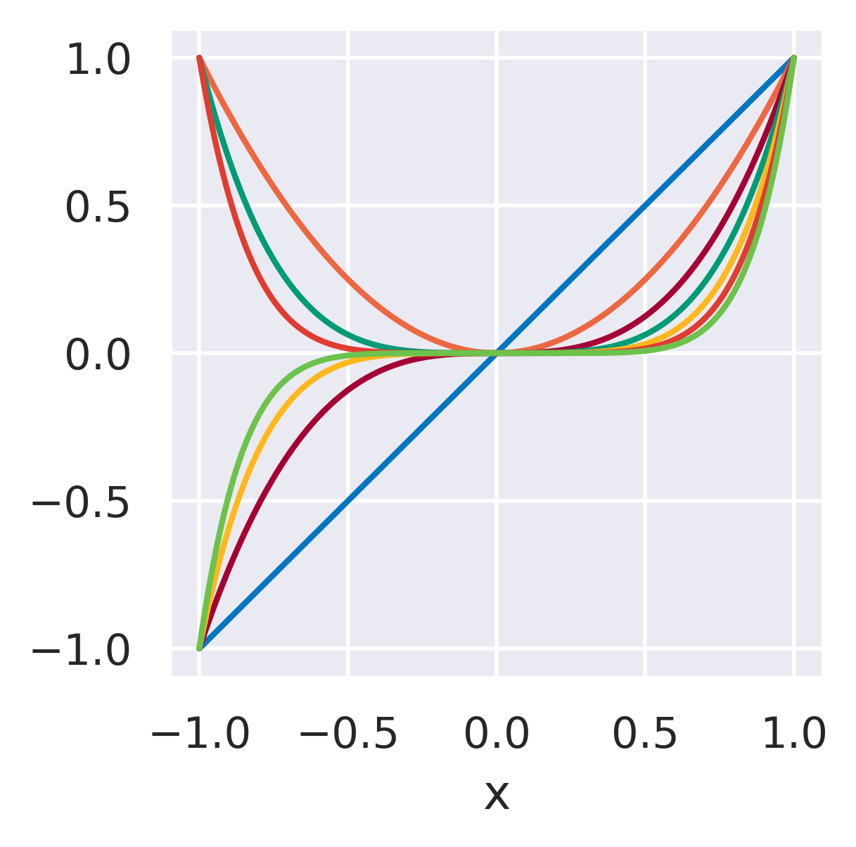
\(\phi_j=x^j\quad\)
None
Functions with global support
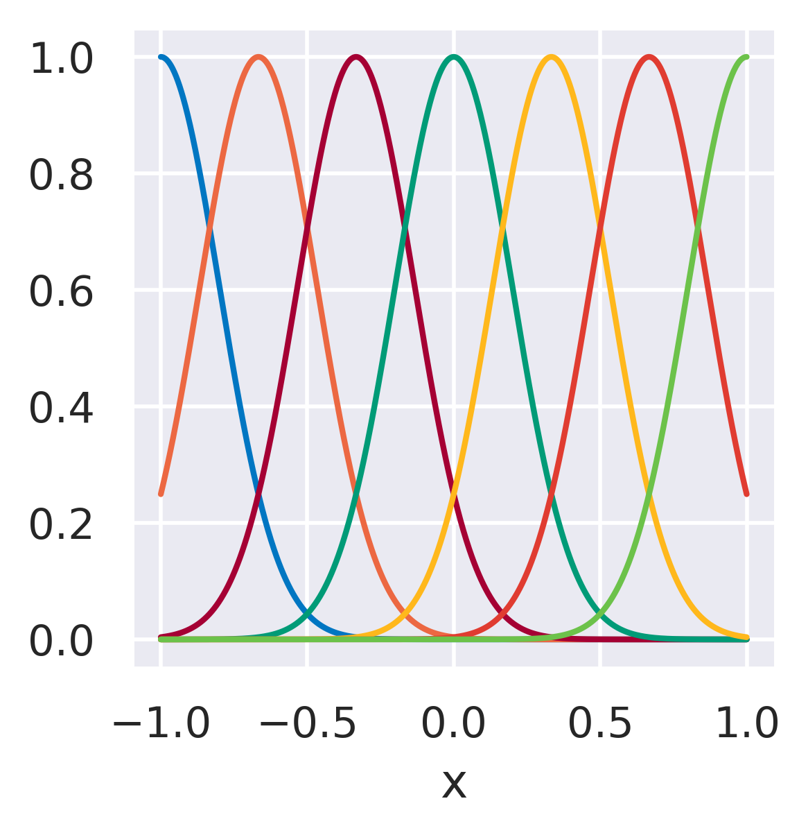
\(\phi_j=\exp\left[-\displaystyle\frac{(x-\mu_j)^2}{2s_j^2}\right]\quad\)
\(\mu_j\): Center of each basis
\(s_j\): Length scale (area of influence)
Functions with localized support, transitions.
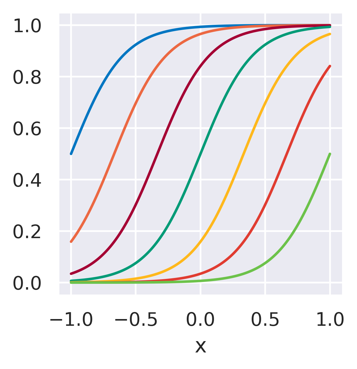
\(\phi_j = \displaystyle\frac{1}{1+\exp\left(\frac{\mu_j-x}{s_j}\right)}\quad\)
\(\mu_j\): Location parameter
\(s_j\): Length scale (area of influence)
Functions whose influence saturate over \(x\)
where we see that they can be nonlinear in \(\mathbf{x}\) while still being linear in \(\mathbf{w}\).
With this we can already define a graph for our model:
Fig. 10 A probabilistic graph for regression.#
Note that \(\mathbf{x}\) is modeled as deterministic here. With this in mind, the joint distribution for this graph is simply:
and we already decided to make \(p(t\vert\mathbf{w},\mathbf{x})\) a Gaussian.
But what to do about \(p(\mathbf{w})\)? At this point we can adopt a prior distribution over it. To make matters simple, let us also assume it is Gaussian:
where we are assuming a prior with zero mean and diagonal covariance. Let us add that to our graph:
Fig. 11 A probabilistic graph for regression, now with hyperparameters.#
and we now also add the \(\beta\) parameter from the observation model. Since they govern the shapes of our distributions but not the actual values of \(\mathbf{w}\), we say \(\alpha\) and \(\beta\) are hyperparameters.
Our model is in principle ready to be used. But since the above prior is not very informative, we first need to observe some data to get a better idea of what the weights actually are.
Observing some data#
Suppose we now observe \(N\) samples of \(t\) values and their associated \(\mathbf{x}\) values. We gather these observations in a matrix \(\mathbf{X}=\left[\mathbf{x}_1,\dots,\mathbf{x}_N\right]\) and a column vector \(\mathbf{t}=\left[t_1,\dots,t_N\right]^\mathrm{T}\).
This changes our graph to:
Fig. 12 A probabilistic graph for regression, now with observations.#
where the plate with the \(N\) inside means we should imagine these two nodes repeated \(N\) times.
Assuming these \(N\) observations are made independently and identically distributed (i.i.d.) from \(p(t\vert\mathbf{w},\mathbf{x})\), we can get a joint distribution for our whole dataset:
We are now standing at a crossroads. We can either take a shortcut and get a single estimate for \(\mathbf{w}\) or we can go fully Bayesian and compute the posterior with:
Two deterministic shortcuts to \(\mathbf{w}\)#
First we take two possible shortcuts to a quick estimate for the weights. We also discuss why they are not always a good choice.
For the first one we note that Eq. (40) is a multivariate Gaussian for \(\mathbf{t}\) (the product of two or more Gaussians is also a Gaussian). We can therefore go the frequentist way:
Maximum Likelihood Estimation (MLE)
Given a likelihood function \(p(\mathbf{t}\vert\mathbf{w})\), compute \(\mathbf{w}\) that maximizes this likelihood. The prior over \(\mathbf{w}\) is ignored and only a single point estimate \(\mathbf{w}_\mathrm{MLE}\) remains.
Taking the logarithm of Eq. (40) turns the product into a sum and gets rid of the exponentials inside (recall the form of a univariate Gaussian):
Note the term in red above. Maximizing Eq. (42) is exactly equivalent to minimizing this term. We therefore get the least squares solution from frequentist regression. Recall that this works well when we have a lot of data but tends to overfit to small datasets.
The second shortcut already uses Eq. (41), so it is a better compromise, although it is still a single point estimate for the weights:
Maximum A Posteriori (MAP)
Given a likelihood and a prior, use Bayes’ theorem to compute a posterior \(p(\mathbf{w}\vert\mathbf{t})\) but keep only the most likely value of \(\mathbf{w}\) as estimate. The prior is taken into account but the uncertainty associated with \(\mathbf{w}\) is ignored.
To get a MAP estimate from Eq. (41) it suffices to look at the numerator (the unnormalized posterior). Taking the logarithm and isolating only what depends on \(\mathbf{w}\) we have:
Getting the most likely value for \(\mathbf{w}\) means maximizing the expression above. Now compare this to the expression for regularized least squares you have seen before, especially the term in red. The MAP solution is exactly equivalent to least squares with \(L_2\) regularization!
These results are quite neat, as they unify all the regression approaches we have seen thus far.
Further Reading
Make sure you understand how MLE, MAP and the Bayesian posterior for \(\mathbf{w}\) are related to each other. Reading Section 3.2 and the first two pages of Section 3.3 will give you a different flavor of this same discussion.
bishop-prml
The Bayesian way#
Finally, we can get a proper probability density for \(p(\mathbf{w}\vert\mathbf{t})\) by using the Bayes’ theorem in Eq. (41) consistently. Note that the likelihood \(p(\mathbf{t}\vert\mathbf{w})\) is a conditional Gaussian, \(p(\mathbf{w})\) is a marginal Gaussian, and the joint distribution (the numerator) is also Gaussian. This means we can directly use the standard expressions we derived before to easily derive a posterior:
where the mean of the posterior is:
and its covariance:
where \(\Phi_{ij} = \phi_j(x_i)\) already appeared in the MLE treatment.
Making new predictions#
We are almost done! We now have a more informed distribution \(p(\mathbf{w}\vert\mathbf{t})\). All that remains now is to finally make new predictions.
Suppose we now have a new input value \(\hat{\mathbf{x}}\) and we would like to predict \(\hat{t}\). We make one final change to our graph:
Fig. 13 A probabilistic graph for regression, final version.#
The joint distribution for this final graph is:
Conditioning on \(\mathbf{t}\) makes the posterior over \(\mathbf{w}\) appear:
And finally we can get the distribution over \(\hat{t}\) by marginalizing \(\mathbf{w}\) out:
Considering for a moment only \(\mathbf{w}\) and \(\hat{t}\), we now have a joint Gaussian with a marginal \(p(\mathbf{w}\vert\mathbf{t})\) and a conditional \(p(\hat{t}\vert\mathbf{w})\) and we want the marginal \(p(\hat{t})\). Using again the standard expressions, we get:
where \(\mathbf{m}\) and \(\mathbf{S}\) come directly from Eqs. (45) and (46).
Further Reading
Read Section 3.3.2 for more details on this predictive distribution. Study what the two terms of the predictive variance represent, and what happens to them in Figure 3.8.
bishop-prml
Click below to see three different radial basis function models fitted to the same dataset using the three strategies we discussed.
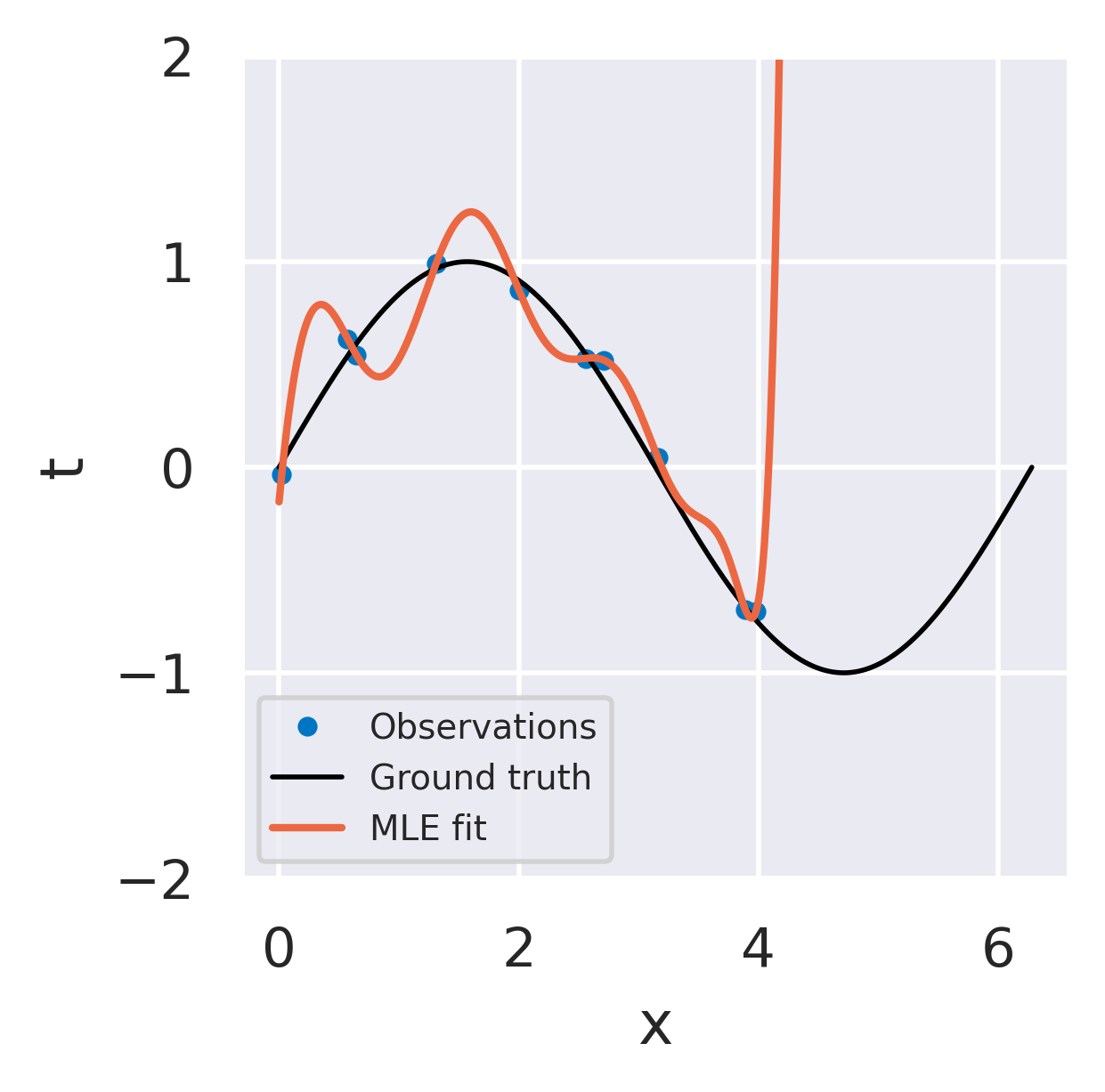
Unregularized least squares fit
No uncertainty information
Overfits noise in data
Response explodes in extrapolation
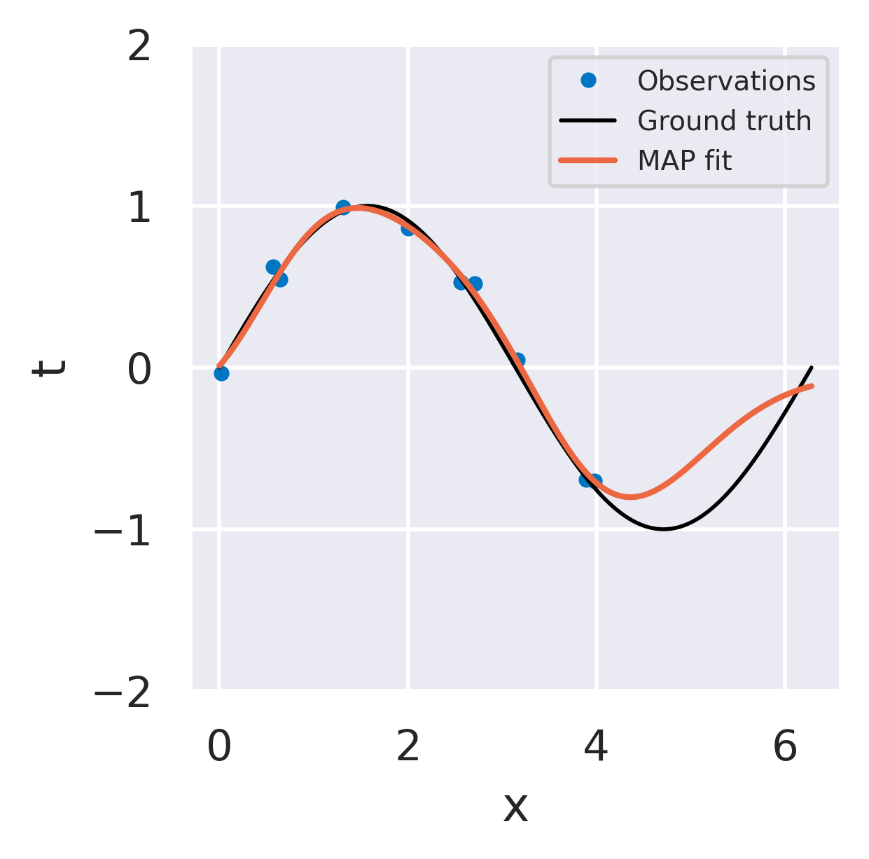
Regularized (\(L_2\)) least squares fit
No uncertainty information
Regularization prevents overfitting
Behaves well away from observations
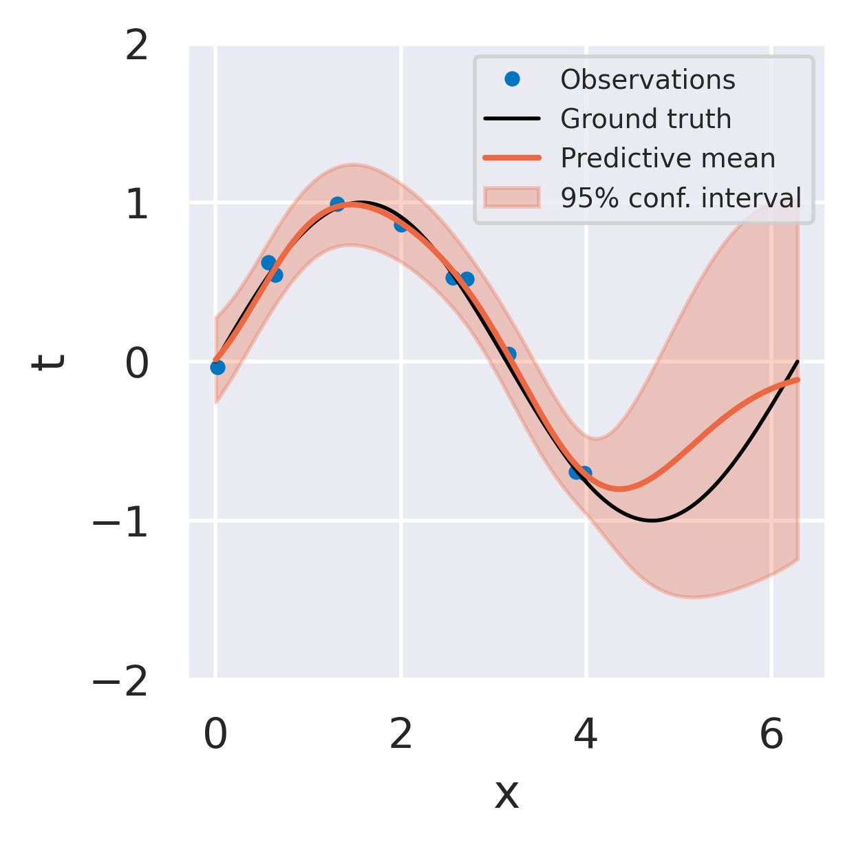
Consistent Bayesian fit
Provides uncertainty information
Prior distribution prevents overfitting
Variance increases away from data
