Distributed load

Distributed loads are loads which are defined per unit length / area / volume. In planar systems, only line loads exist, generally specified with the symbol \(q(x)\) with the unit \(\text{kN/m}\). \(q(x)\) can be any function, although linear functions are most apparent.

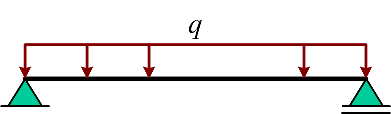
An example of a constant distributed load with unknown value \(q\) is shown in the figure below:

Finding resulting force of distributed line load

The resulting force can be calculated with:

()\[R = \int\limits_{{x_1}}^{{x_2}} {q\left( x \right)dx}\]

it works on a distance \(x_R\) from the axis:

()\[x_R = {{\int\limits_{{x_1}}^{{x_2}} {x{\mkern 1mu} {\kern 1pt} q\left( x \right)dx} } \over {\int\limits_{{x_1}}^{{x_2}} {q\left( x \right)dx} }}\]

For constant loads (\(q(x)\) is constant), equation () simplifies to \(R = q \cdot L\) with \(L\) the length over which the load \(q\) is present. This load \(R\) acts halfway the length \(L\) according to ().

For triangular loads, equations () and () simplifies to \(R = {1 \over 2}q_\text{max} \cdot L\) with \(R\) acting at \({1 \over 3} L\) from the points for which \(q\) is at it’s maximum.

Finding resulting force of distributed field load

The resulting force can be calculated with:

()\[R = \int\ {p\left( x, y \right)dA}\]

it works on a distance \(x_R\) and \(y_R\) from the axis:

()\[x_R = {{\int\ x {\kern 1pt} {p\left( x, y \right)dA} } \over {q\left( x \right)dA} }, y_R = {{\int\ y {\kern 1pt} {p\left( x, y \right)dA} } \over {q\left( x, y \right)dA} }\]

Example video

Practice material

• If you’re a TU Delft student, you can practise using the Dutch exercises on ANS. Every time you open this link you get a new exercise.

• Additional exercises are available in chapter 6.6 of the book Engineering Mechanics Volume 1 in chapter 6 [Hartsuijker and Welleman, 2006].

Relation with other subjects

Additional reading

Lecture slides

The lecture slides of the relevant lectures at Delft University of Technology are available here.

Book

The content can be found in the book Engineering Mechanics Volume 1 in chapter 6 [Hartsuijker and Welleman, 2006].