Example incremental method lecture 3 plasticity

The following structure is investigated

#import packages
import sympy as sym
import matplotlib.pyplot as plt
sym.init_printing()

#Defines symbols and functions
EI, q_L, x, L, M_p = sym.symbols('EI, q_L, x, L, M_p')
w = sym.Function('w')

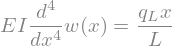
# Define the ODE for the bending of the beam
ODE_bending = sym.Eq(w(x).diff(x, 4) *EI, q_L/L*x)
display(ODE_bending)

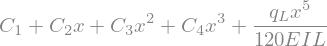
# Solve the ODE
w = sym.dsolve(ODE_bending, w(x)).rhs
display(w)

# Define the continuum fields of phi, kappa, M, and V
phi = -w.diff(x)
kappa = phi.diff(x)
M = EI * kappa
V = M.diff(x)

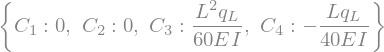
Linear behaviour: fixed beam at both ends

# Define the boundary conditions
eq1 = sym.Eq(w.subs(x,0),0)
eq2 = sym.Eq(w.subs(x,L),0)
eq3 = sym.Eq(phi.subs(x,0),0)
eq4 = sym.Eq(phi.subs(x,L),0)

# Solve the integration constants
sol1 = sym.solve([eq1, eq2, eq3, eq4 ], sym.symbols('C1, C2, C3, C4'))
display(sol1)

# Define some dummy values to plot the results
plotvalues = {EI:1, q_L:1, L:1, M_p:0.01}

# Plot the moment line to identify the maximum moment
sym.plot(-M.subs(sol1).subs(plotvalues),(x,0,1),ylabel='M(x)',title='Moment line');

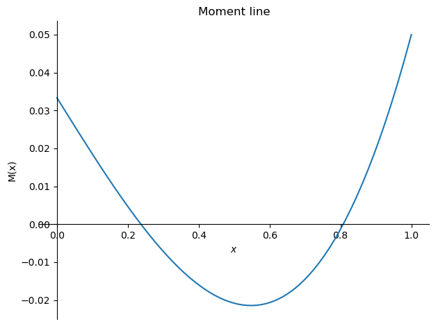
# Obtain the maximum moment at x = L
display(M.subs(sol1).subs(x,L))

# Obtain the load corresponding to the first yield moment
q1 = sym.solve(sym.Eq(-M.subs(sol1).subs(x,L),M_p), q_L)[0]
display(q1)

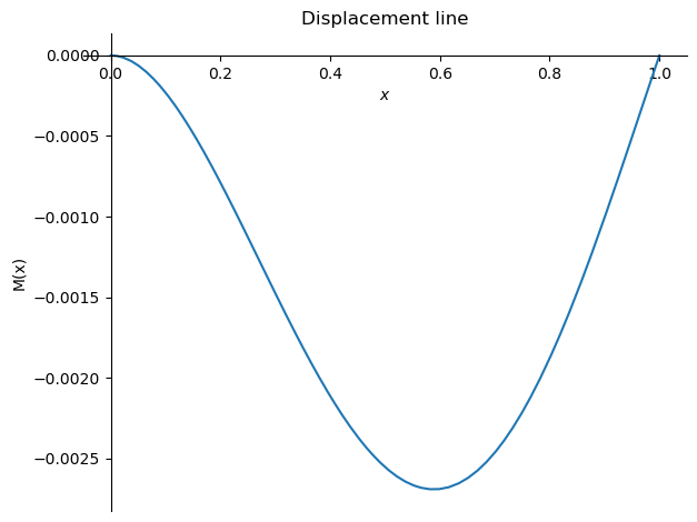
# Plot the displacement line
sym.plot(-w.subs(sol1).subs(plotvalues),(x,0,1),ylabel='M(x)',title='Displacement line');

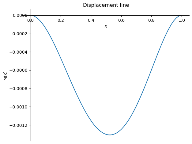
# Obtain the displacement at x = L/2
w1 = w.subs(sol1).subs(q_L, q1).subs(x,L/2)
display(w1)

Plastic behaviour: Beam simply supported on right with \(M_p\) working at it

# Define the boundary conditions
eq1 = sym.Eq(w.subs(x,0),0)
eq2 = sym.Eq(w.subs(x,L),0)
eq3 = sym.Eq(phi.subs(x,0),0)
eq4 = sym.Eq(M.subs(x,L),-M_p)

# Solve the integration constants
sol2 = sym.solve([eq1, eq2, eq3, eq4 ], sym.symbols('C1, C2, C3, C4'))
display(sol2)

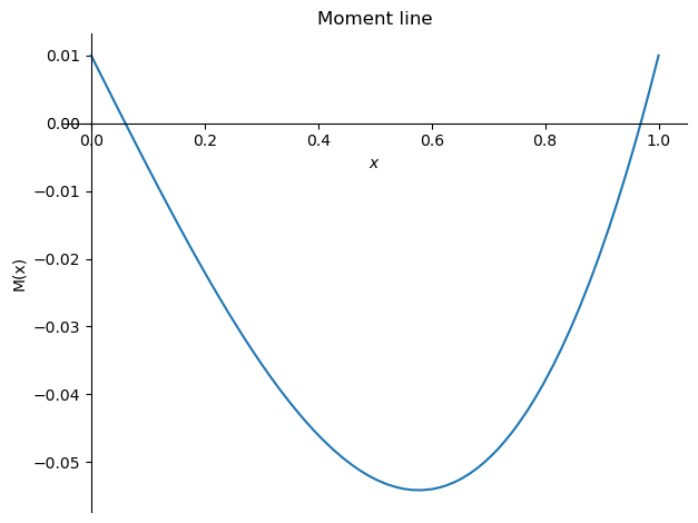
# Plot the moment line to identify the maximum moment
sym.plot(-M.subs(sol2).subs(plotvalues),(x,0,1),ylabel='M(x)',title='Moment line');

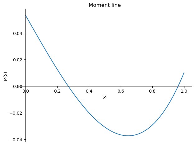
# Obtain the maximum moment at x = 0
display(M.subs(sol2).subs(x,0))

# Obtain the load corresponding to the second yield moment
q2 = sym.solve(sym.Eq(-M.subs(sol2).subs(x,0),M_p), q_L)[0]
display(q2)

# Plot the displacement line
sym.plot(-w.subs(sol2).subs(plotvalues),(x,0,1),ylabel='M(x)',title='Displacement line');

# Obtain the displacement at x = L/2
w2 = w.subs(sol2).subs(q_L, q2).subs(x,L/2)
display(w2)

Plastic behaviour: Beam simply supported on both ends with \(M_p\) working at it

# Define the boundary conditions
eq1 = sym.Eq(w.subs(x,0),0)
eq2 = sym.Eq(w.subs(x,L),0)
eq3 = sym.Eq(M.subs(x,0),-M_p)
eq4 = sym.Eq(M.subs(x,L),-M_p)

# Solve the integration constants
sol3 = sym.solve([eq1, eq2, eq3, eq4 ], sym.symbols('C1, C2, C3, C4'))
display(sol3)

# Plot the moment line to identify the maximum moment
sym.plot(-M.subs(sol3).subs(plotvalues),(x,0,1),ylabel='M(x)',title='Moment line');

# Find the location of the maximum moment
x_M_max = sym.solve(sym.Eq(V.subs(sol3),0),x)[1]
display(x_M_max)

# Obtain the maximum moment at x = x_M_max
display(M.subs(sol3).subs(x,x_M_max))

# Obtain the load corresponding to the third yield moment
q3 = sym.solve(sym.Eq(M.subs(sol3).subs(x,x_M_max).subs(x,0),M_p), q_L)[0]
display(q3)

# Plot the displacement line
sym.plot(-w.subs(sol3).subs(plotvalues),(x,0,1),ylabel='M(x)',title='Displacement line');

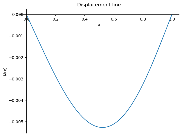
# Obtain the displacement at x = L/2
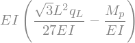
w3 = w.subs(sol3).subs(q_L, q3).subs(x,L/2).simplify()
display(sym.simplify(w3))

Mechanism: Beam simply supported on both ends with \(M_p\) working at it and a plastic hinge at \(\frac{\sqrt{3}L}{3}\)

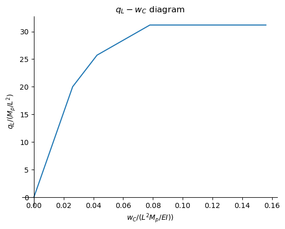
\(q_L-w_C\) diagram

# Obtain the displacements and q values as coefficients of a constant term.
w_list = [0,w1.coeff(L**2*M_p/EI),w2.coeff(L**2*M_p/EI),w3.coeff(L**2*M_p/EI),w3.coeff(L**2*M_p/EI)*2]
q_list = [0,q1.coeff(M_p/L**2),q2.coeff(M_p/L**2),q3.coeff(M_p/L**2),q3.coeff(M_p/L**2)]

# Plot the q_L-w diagram
plt.plot(w_list,q_list)
plt.xlabel('$w_C / (L^2 M_p / EI))$')
plt.ylabel('$q_L / (M_p / L^2)$')
plt.title('$q_L-w_C$ diagram')
plt.gca().spines['right'].set_color('none')
plt.gca().spines['top'].set_color('none')
plt.gca().spines['bottom'].set_position('zero')
plt.gca().spines['left'].set_position('zero')