Live Code (Sphinx Thebe)#
The live-coding option is what makes working with these interactive textbooks extra attractive for courses where coding might be involved or useful to showcase examples. Additionally, it is useful to illustrate the content in a way which the student will recognize during programming assignments.
This page will show some examples where live coding is used in combination with theoretical questions as well as as stand-alone exercises used to round off a theoretcal chapter with a practical application.
Python for Engineers#
Python for engineers is a book used to introduce basic programming concepts to students coming from different universities where programming is not a big part of the curriculum like at TU Delft. The students are encouraged to follow the course online before the start of the year to hit the ground running in September. Chapter 7 introduces the students to Matplotlib and teaches them various ways of making a graph.
Live coding is the perfect learning tool as the students can see how the code relates to the visual result of the graph. subsequently, they can adapt the code and observe the changes. Let’s have a look at the implementation.
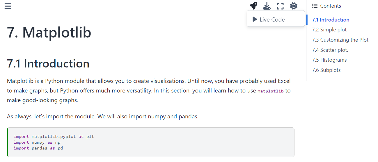
Fig. 71 Rocket Button#
To activate the live coding, the rocket button has to be activated like in the figure above. It’s always useful to point this out in the beginning of the chapter because it might not be obvious to new users. Here’s a not eused in the MUDE book
This online textbook has a number of pages that are set up to be used interactively. You can use the “Live Code” button under the Rocket Ship icon in the top right to activate the interactive features and use Python interactively!

Sometimes the interactivity will involve completing an exercise, wheras on other pages it might simply provide the opportunity to edit the contents of code cells and execute it to explore the page contents interactively. Other pages may provide interactive figures (e.g., widgets).

This feature is supported by TeachBooks.
Once the live coding is activated the code cells run the python code. They even display error messages if there is a mistake in the code.
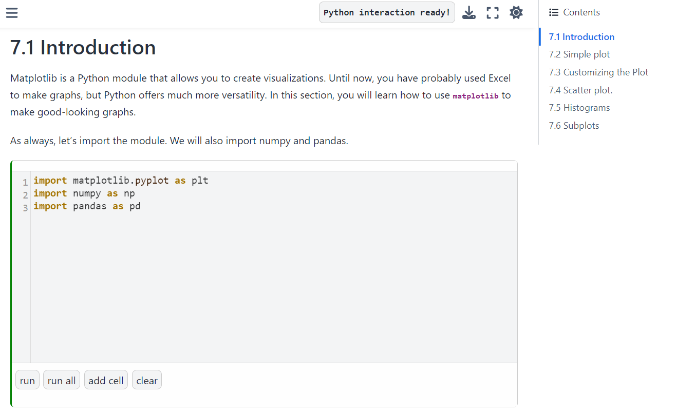
Fig. 72 Python Ready#
After introducing some types of plots and breaking down and explaining the lines of code, it is time for the student to have little go themselves. The code is given and they can customize the input.
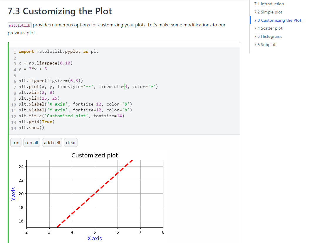
Fig. 73 Graph Customization#
This example is rather basic but a similar concept can be applied to more difficult concepts in engineering. The student is getting direct feedback from the code to see how a different input changes the output which reinforces the theory.
MUDE - Signal Processing#
In MUDE, the concept of Signal Processing is introduced. On top of the theory, a working example is used to test the understanding of the students. When talking about Signal Processing, the Fourier Series is a foundational block that has to be well understood. The fourier series is used to describe basically any periodic function/signal as a sum of multiple cosines and sines with different frequencies. This is illustrated with the concept of the square wave.
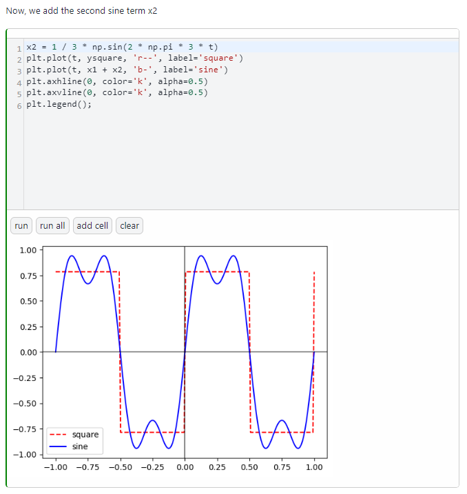
Fig. 74 Superposition of two signals#
By adding more signals themselves, the students will see that the fourier series approximates the square wave. They might even see which frequencies work better than others.
Finally lets look at a more computationally heavy example.
MUDE - Machine Learning#
In the chapter on the k-nearest neighbour, live-coding is activated by default in order to run all the coding which supports the theory. For more complex topics, it is useful to keep the actual code cells hidden and only display the graphs with interactive sliders in order to focus the learning objective more on the content and less on the coding.
The k-nearest neighbour method predicts the value f(x) for a given x by taking the average value of its neigbhours and assigning it to f(x). The amount of neighbours considered is governed by the variable k.

Fig. 75 Interactive Graph#
Multiple sliders modify the predicted graph (in orange) by taking into account a different amount of neighbours, training size, frequency of the signal and amount of noise. The student is able to verify the claims made by the theory throught the interactive graph.