Curve-fitting

Click –> Live Code to activate live coding on this page!

Problem

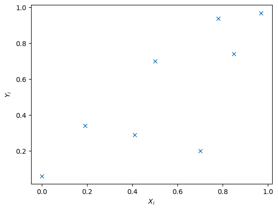
8 data points are collected where \(X_i\) is the explanatory variable and \(Y_i\) the response variable. It is believed that the data follows the trend \(Y = aX^b+c\) where \(a\), \(b\) and \(c\) are the parameters to be determined to fit the model.

\(X_i\)	\(Y_i\)
0.97	0.97
0	0.06
0.5	0.7
0.85	0.74
0.7	0.2
0.19	0.34
0.41	0.29
0.78	0.94

Fig. 1.2 8 data points

Examples of the source of this data can be:

• Stress of a pre-stressed concrete specimen based on the deformation when applied an axial force

• Permeability-coefficient for compacted sand based on the grain size

• Job performance based on the number of working hours

• etc.

Model

We need to define our problem in the form of unconstrained optimization (1.1).

The problem is modelled as a minimization of the squared error, where error is the difference between \(a X_i^b+C\) and \(Y_i\)

(1.3)\[\mathop {\min }\limits_{a,b,c} \sum\limits_{i = 1}^8 {{{\left( {a{X_i}^b + c - {Y_i}} \right)}^2}}\]

Find best solution manually

Test yourself

Try and adjust the values for \(a\), \(b\) and \(c\). How small can you get the total error squared?

Method

Again, this model is described using scipy.optimize.minimize according to the standard structure in this course

Import libraries

import scipy as sp
import numpy as np
import matplotlib.pyplot as plt

import scipy as sp
import numpy as np
import matplotlib.pyplot as plt

Define the variables

In this problem, there are 3 design variables: \(a\), \(b\) and \(c\). In scipy.optimize, these variables are part of one array. You don’t have to specify this variable beforehand, but the optimization algorithm will define the number of variables on your other input. Furthermore, input data is given which is required to specify explicitly. Additionally, an initial guess is required for the otimization algorithm.

xi = np.array([0.97, 0   , 0.5, 0.85, 0.7, 0.19, 0.41, 0.78])
yi = np.array([0.97, 0.06, 0.7, 0.74, 0.2, 0.34, 0.29, 0.94])
abc0 = np.array([4., 2., 0.5]) #initial guess

Define objective function

The objective function was defined in (1.3). Because a, b, c and xi are all numpy arrays, we can simply use *, ** and + to deal with the multiplication, exponent and summation of those arrays. np.sum is used to sum up all components of the array which is the result of (yi-y_est)**2

def squarederror(abc):
    a = abc[0]
    b = abc[1]
    c = abc[2]
    y_est = a * xi ** b + c
    error = np.sum((yi-y_est)**2)
    return error

Solve the problem

Now we can solve the actual problem

result2 = sp.optimize.minimize(squarederror,abc0)
print(result2)

  message: Optimization terminated successfully.
  success: True
   status: 0
      fun: 0.33422039804882037
        x: [ 8.028e-01  1.231e+00  1.233e-01]
      nit: 22
      jac: [-8.419e-07  1.155e-07 -1.021e-06]
 hess_inv: [[ 6.553e-01 -4.265e-01 -3.822e-01]
            [-4.265e-01  1.800e+01  2.730e+00]
            [-3.822e-01  2.730e+00  6.355e-01]]
     nfev: 96
     njev: 24

Test yourself

Postprocess results

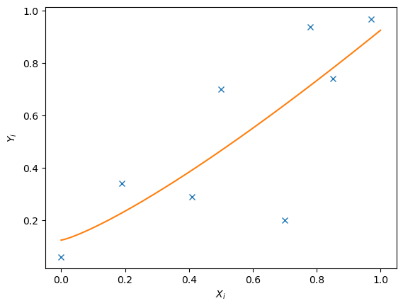
As this problem involves three design variables, a plot of all possible design variables with the objective function is not possible because it would require four dimensions. However, we can plot the data which the obtained solution to see how it looks like

x_range = np.linspace(0,1,100)
plt.plot(xi,yi,'x');
plt.plot(x_range,result2.x[0] * x_range ** result2.x[1] + result2.x[2])
plt.xlabel('$X_i$')
plt.ylabel('$Y_i$');

Exercise

Test yourself

Click –> Live Code and adapt the code to answer the following question.

Questions, discussions and comments