Bathymetry maps#
Click –> Live Code to activate live coding on this page!
Problem#
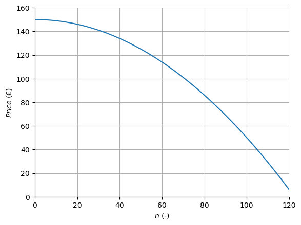
It is desired to determine the number of bathymetry maps \(n\) of a local area that should be produced to maximize the profit of a company. The total cost of production and distribution is €\(75\) per unit \(n\). The revenues are proportional to the number of units multiplied by its price: \(Revenues = n \cdot Price \)
The demand depends on the price (\(n = \sqrt{100 \cdot \left(Price - 150 \right)}\)), as shown in the graph:
Show code cell source
import numpy as np
import matplotlib.pylab as plt
%config InlineBackend.figure_formats = ['svg']

n = np.linspace(0,125,100)
price = 150 - 0.01 * n**2
plt.plot(price,n)
plt.ylabel('$n$ (-)')
plt.xlabel('$Price$ (€)')
plt.xlim(0,160)
plt.ylim(0,130)
ax = plt.gca()
ax.grid(True, which='both')
ax.spines['left'].set_position('zero')
ax.spines['right'].set_color('none')
ax.yaxis.tick_left()
ax.spines['bottom'].set_position('zero')
ax.spines['top'].set_color('none')
ax.xaxis.tick_bottom()

Fig. 1.1 \(Price = 150 - 0.01n^2\)#
The profit can be estimated as the revenues minus the total costs.
Model#
We need to define our problem in the form of unconstrained optimization (1.1).
The function for the profit can be found by combining the relations in the problem statement. However, this is the profit which should be maximized. To turn this into a minimization problem, the profit can be multiplied with \(-1\). The final model of this problem results in:
Find best solution manually#
An approach to solve this problem might be to try out some values. You can do so in the applet below. The plot below shows the negative profit for some number of bathmetry maps sold.
Try and adjust the values for \(n\), the number of bathmetry maps sold. How small can you get the negative profit?
As this case is only one-dimensional and the potential range of values is limited, this approach (exhaustive search) is valid: evaluating all possible values for \(n\) doesn’t take a lot of computing power. The resulting values from the objective function show a clear minimum. For problem in which the objective function required more computational power or the amount of dimensions of the design variables increases, this approach quickly becomes infeasible.
Method#
Now let’s solve this problem using an optimization method. This model is described using scipy.optimize.minimize according to the standard structure in this course
Import libraries#
For this problem, we’ll use all three packages scipy, numpy, matplotlib.
import scipy as sp
%config InlineBackend.figure_formats = ['svg']
import scipy as sp
import numpy as np
import matplotlib.pylab as plt
Define the variables#
There are very few variables in this problem. In fact, the only variable we have to specify is the initial guess for the optimization algorithm. The objective function will be treated later. The length of \(n\) doesn’t have to be specified.
n0 = 20
Define the objective function#
In the objective function, the formula derived above in (1.2) ean be inserted. Or, each individual step can be calculated on a seperate line. Again, note that the profit is multiplied with \(-1\) to maximize the profit in the minimization formulation. This results in:
def negprofit(n):
    price = 150 - 0.01 * n**2
    revenues = price * n
    totalcost = 75 * n
    profit = revenues - totalcost
    return -profit
Solve the problem#
Now, the problem can be solved. The result is stored in the variables result which is printed.
result = sp.optimize.minimize(negprofit,n0)
print(result)
  message: Optimization terminated successfully.
  success: True
   status: 0
      fun: -2499.9999999998727
        x: [ 5.000e+01]
      nit: 8
      jac: [ 0.000e+00]
 hess_inv: [[ 3.503e-01]]
     nfev: 22
     njev: 11
Postprocess results#
As seen before, this problem is very small and can be solved by evaluating all possible values (or applying algebra). These values can be plotted and the optimum solution is clearly in the minimum.
n_range = np.linspace(0,100,100)
negprofit_result = negprofit(n_range)
plt.figure()
plt.plot(n_range,negprofit_result)
plt.plot(result.x,result.fun,'o');
plt.xlabel('$n$')
plt.ylabel('Negative profit');
ax = plt.gca()
ax.spines['right'].set_color('none')
ax.spines['top'].set_color('none')
ax.spines['bottom'].set_position('zero')
ax.spines['left'].set_position('zero')
Exercise#
Click –> Live Code and adapt the code to answer the following question.
